TS-CHEM Solution Library - AT123D-AT

The TS-CHEM program provides an easy-to-use software environment in which to analyze contaminant plume transport, and includes a comprehensive library of more than 30 different analytical solutions to the advection-dispersion equation. Each solution incorporates different capabilities, including how it represents the contaminant source and how the plume interacts with the aquifer. For this post in the Solution Library series, we will be focusing on the AT123D-AT family of models published by Dan Burnell in 2012 which represents an updated version of the original AT123D model suite developed by G.T. Yeh at the Oak Ridge National Laboratory.

What is AT123D?

The original AT123D was a suite of analytical model solutions that are used to simulate one-, two- and three-dimensional transport in groundwater. The program is complex, and allows for many different source configurations, including

• patch sources
• line sources
• point sources
• volume sources

In contrast to many analytical plume models that represent the source using a first-type specified concentration, AT123D represents the source as a second-type specified mass flux boundary condition. This means, for example, if you know the nitrogen load from a residential dwelling to a septic system (i.e. number of residents times average daily nitrogen load per person) you can represent that source in AT123D as milligrams of nitrogen per day instead of trying to estimate a septic source concentration value. The primary difference between AT123D and AT123D-AT is in how the solver arrives at a solution to the advection-dispersion equation. AT123D-AT incorporates a Romberg numerical integration scheme that works to prevent oscillations, speed convergence, and improve accuracy for a wide range of input parameter combinations.

A conceptualization of the many possible specified mass flux source geometries available in AT123D-AT is shown in Figure 1 below, and can also be found in the Model Selection Tool in TS-CHEM:

Figure 1 - AT123D-AT Source Geometries

TS-CHEM was developed with usability in mind, so the numerous AT123D-AT solutions available to the user (differing aquifer geometries, source geometries, and source types) have been broken up into six “versions” (see table below). These pre-configured versions allow the user to select the type of AT123D-AT model that will best represent their site (aquifer and source), and to specify the desired parameter input values to represent site-specific properties, using model types that closely match conditions simulated by other analytical ADE solutions included in ­TS-CHEM’s Solution Library. This last consideration makes it easier to compare different plume transport solutions (e.g. a first-type source vs a second-type source) by selecting similar type models (e.g. with aquifer boundaries or without aquifer boundaries) from the TS-CHEM Solution Library.

The following nomenclature is used between each version to help the user quickly determine which version they are looking for: Infinite boundary (I), Finite boundary (F), Constant mass release rate (C), Instantaneous release source (I), Time-variable (transient) mass flux (T):

Model Version	Aquifer Boundary	Source Type	Analagous TS-CHEM models
AT123D-AT IC	Infinite unbounded	Constant mass flux	3DADE-3 or 3DADE-4 (patch source)
AT123D-AT II	Infinite unbounded	Initial mass instantaneous release	3DADE-5 or 3DADE-6 (volume source)
AT123D-AT IT	Infinite unbounded	Constant specified concentration	ATRANS4 (with concentration stepping)
AT123D-AT FC	Finite bounded	Constant mass flux	ATRANS1
AT123D-AT FI	Finite bounded	Initial mass instantaneous release	3DADE-5 or 3DADE-6 (volume source)
AT123D-AT FT	Finite bounded	Constant specified concentration	ATRANS4 (with concentration stepping)

What are the differences between the AT123D-AT models?

The two defining factors that highlight the differences between the different AT123D-AT models are 1) whether the aquifer extent is assumed to be infinite (as is the case for many analytical transport solutions) or finite (bounded horizontally or vertically), and 2) how the source concentration or flux is applied at the model boundary over time (continuous, instantaneous pulse release, or time-varying). The three different types of source concentration fluxes are conceptualized in Figure 2 below:

Figure 2 - AT123D-AT Model Source Types

As you can see in Figure 2, there are three distinct source types. The source type that is most appropriate to use in a particular application is dependent on the known conditions at a site, and/or the known or assumed conditions of the source.

What applications are the AT123D models best suited for?

As discussed in previous blog posts, TS-CHEM can assist environmental professionals with the development of conceptual site models (CSMs) that characterize the extent and behavior of groundwater contaminant plumes. The AT123D-AT models are highly flexible, able to provide users with the ability to evaluate solute fate and transport in one-, two- or three-dimensions. In its fundamental form, AT123D-AT is solving the 3D ADE equation in a 1D (X-direction only) aquifer flow field, but 2D plume transport and even 1D “column” transport can be set up using the bounded aquifer settings. i.e. the AT123D-AT “F” models (FC, FI, and FT) can be used to represent sites where the aquifer thickness and/or width is known or is believed to be bounded (finite aquifer boundary). This type of AT123D-AT model is similar to the ATRANS family of models which include an upper (water table) and lower (aquifer base) no-mass-flux boundary.

But the AT123D-AT models are not all limited to bounded aquifer conditions. The AT123D-AT “I” models (FI, II, and IT) can be used to represent sites where there is no limitation on aquifer thickness or width (infinite aquifer boundary). This type of AT123D-AT model is similar to the 3DADE family of models, which do not impose any finite boundaries on the aquifer.

Further, the investigator can use a variety of patch source geometries to best represent the conditions at their site. For example, if an investigator has information on source mass flux at the downgradient edge of a source area, they may use a patch source. Or, if a large regional scale model is being considered, the user may want to utilize a point source to track the general plume behavior over time.

When choosing between source types, a user may choose to use a constant mass release source AT123D-AT model If only a single source concentration is known, and/or the investigator wished to perform a conservative analysis in which the source does not deplete through time. If the user wanted to investigate the plume behavior in a case where a slug of solute is introduced into the groundwater, they can use an instantaneous release source type. If information is available on the changing history (both increases and decreases) of source flux over time, the transient source type can be used.

Similar to the ATRANS1 model, the AT123D-AT FC model is useful for simulating scenarios that have aquifers of a finite extent that can be represented by a continuous mass flux. This type of analysis may be useful for evaluating a conservative maximum plume extent, or when the plume becomes stable (Figure 3):

Figure 3 - AT123D-AT FC solution showing maximum plume extent for a stable benzene plume with a constant source flux of 0.001 ld/d at 200ft, 600ft and 1000ft from the source.

The AT123D-AT FI model is useful for simulating scenarios where a slug of contaminant is assumed to have rapidly entered the groundwater. This type of model is sometimes used in an emergency spill response analysis if an investigator wants to simulate a conservative condition where a “slug” of contaminant enters the groundwater instantaneously and then is allowed to flush away from the spill area toward a possible receptor location (Figure 4):

Figure 4 - AT123D-AT FI solution showing plume concentrations up to 4000 days after an instantaneous mass input of 22.05 lbs of benzene introduced to groundwater. Concentrations are shown at 200ft, 600ft and 1000ft from the source. 

Similar to the ATRANS4 model, the AT123D-AT FT model allows the user to define transient source behavior. Unlike ATRANS4, the AT123D-AT FT model uses a second-type boundary condition and is therefore defined by time-flux pairs (instead of time-concentration pairs). The transient source condition allows the user great flexibility in how they define the time series of their source and can enable investigators to simulate complex scenarios where there may be intermittent single sources, multiple sources that overlap at different times, or even source termination that would result from remedial actions.

An example of a time-variable source flux is shown in Figure 5 below for a hypothetical release from an underground storage tank (UST). The benzene source progressively decreases until it eventually reaches zero after 2000 days. This might be indicative of a UST that leaks over time, or it could be indicative of a UST removal at around 500 days with a small amount of product remaining after removal. In either case, the benzene concentration is reduced over time through degradation/natural attenuation and flushing.

Figure 5 - AT123D-AT FT solution showing benzene plume concentrations entering groundwater from a hypothetical underground storage tank at 200ft, 600ft and 1000ft from the source.

To summarize: the AT123D-AT family of models available in the TS-CHEM Solution Library allow for a very flexible representation of the source over space and through time and can be used for a variety of environmental scenarios and conditions. The feature that sets the AT123D-AT models apart is that they are the only models in the TS-CHEM solution library that utilize a second-type (specified mass flux) source boundary condition, allowing for users to directly input an estimate of source mass flux for their site. AT123D-AT also differs from AT123D in that it incorporates enhanced solver capabilities that reduce solve times and increase solution accuracy. The six AT123D-AT model types included in TS-CHEM allow a user to easily identify which model is best for their site or application. These models can assume either a finite or infinite aquifer boundary and a multitude of source geometries and source release types.

To learn more about TS-CHEM, or to download a FREE DEMO VERSION of the software, visit the TS-CHEM Website today!

Darcy’s Law Groundwater Velocity and Plume Arrival Time

In his 1999 article titled “On Misuse of the Simplest Transport Model”¹ Ernesto Baca explained why it is not a good idea to calculate the rate of travel of a contaminant plume front, or its time of arrival at a receptor location, using the Darcy’s Law groundwater velocity. The missing factor is dispersion.

Baca noted that the Darcy’s Law velocity equation: 

V = Ki/n

only accounts for advection of the dissolved contaminant. He stated that, by measuring the plume from the source location to the far extent of the tip of the plume, one is implicitly considering both advection and dispersion. Therefore, for a relatively mobile dissolved contaminant being transported by seeping groundwater, the larger the dispersive effects, the more your estimate of arrival time will be off.

The toe of the contaminant plume will arrive earlier (i.e. in less time) that you would predict based on a Darcy’s Law groundwater velocity estimate.

The process is depicted in this video:

The video file is available for download. The video presents an analysis of a relatively mobile (slightly adsorbed and retarded) chemical, is for illustrative purposes only, and does not represent McLane Environmental’s analysis of, nor conclusions regarding, any particular real site or plume.

¹ Baca, E. 1999. On the Misuse of the Simplest Transport Model. Groundwater v 37, no 4, Jul-Aug 1999.

TS-CHEM Example Applications – Natural Source Flushing with MNA

 Monitored Natural Attenuation (MNA) is a remediation method that relies on natural processes to decrease contamination in the soil or groundwater. It is a popular method of remediation since it tends to involve less equipment and labor and therefore, less cleanup costs. 

Scientists typically monitor the contamination at a site to ensure that it is attenuating properly and within a reasonable time period. According to New Jersey’s MNA guidance, the applicability of MNA must be demonstrated by lines of evidence directly or indirectly indicate that natural attenuation processes are occurring. With TS-CHEM, it is simple to establish a clear line of evidence that demonstrates natural attenuation is occurring at your site.

This blog post will cover the second Example Application in the TS-CHEM Example Application series: Natural Source Flushing with MNA. To follow along and review the model files, you can download this example application HERE.

Overview

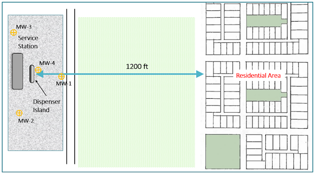
In this scenario, there has been a gasoline release from the dispenser island at a service station. While the leak is repaired shortly after the release, regulators and residents are worried about the release of benzene to the ground considering a residential development is located 1,200 feet to the east where shallow domestic wells are located. An initial on-site investigation reveals the following information:

• Aquifer material = medium sand; some gravel; little silt

• Hydraulic gradient to the east = 0.003 ft/ft

• Source area (MW-4) benzene concentration = 3,000 ug/L

Figure 1. Site map showing the distance from the benzene source at the dispenser island to the residential area.

Concerned by cleanup costs, the responsible party would prefer to remediate the contaminated area using MNA if possible. For MNA to be applicable, the responsible party needs to demonstrate that benzene is being flushed away sufficiently so as not to impact the domestic wells 1,200 feet away. For this example project, the benzene plume boundary is set to 5 ug/L since the USEPA drinking water standard for benzene is 5 ug/L.

Setting Up the Model

Since the leak from the dispenser island has been repaired, there is no constant source of contamination. Because of this, BIOSCREEN-AT is a good model solution for this analysis because its vertical patch source (in a semi-infinite aquifer bounded at the water table)  represents an exponentially decaying source concentration. This model solution will allow you to see changes in maximum plume extent from an early phase of growth, and then through subsequent plume decrease as the sources flushes away. In TS-CHEM, the following model parameters should be set:

• Hydraulic gradient = 0.003 ft/t

• Hydraulic conductivity = 60 ft/d

• Effective porosity = 0.25

• Source width = 10 ft

• Source depth = 2 ft

• Initial Benzene source concentration = 3,000 ug/L

• Initial estimate of source flushing half life = 4 years

Analysis 1: Examining Source Decrease Through Flushing

First, model observation points should be set downgradient from the dispenser at 100 ft (MW-1), 600 ft (mid-way to the neighborhood), and 1000 ft (approaching the neighborhood).

Figure 2. Site map showing model observation points located in between the dispenser island and the residential area.

These observation points should give insight into the levels of benzene at these locations over time and whether the benzene plume is decaying at a sufficient rate. After running the model for ten years, the C v t plots reveal that the plume reaches a peak around 1.5 years on the station property but continues to advance towards the neighborhood. The observation points located farther downgradient from the source show the arrival and growth (increasing concentrations) of the plume until the reduction of the source causes concentrations to decline in these areas.

Figure 3. The C v t chart in TS-CHEM displaying benzene concentrations near the source at MW-1 (dark blue), 600 ft from the source (aqua), and 1000 ft from the source (red).

The contour plot shows that the plume reaches its maximum extent of about 875 feet after 7 years and does not extend into the residential development. The calculated plume at the 7-year time point encompasses an area of  88,350 ft².

Figure 4. TS-CHEM's contour chart indicates that the maximum plume extent (bound at 5 ug/L) does not reach the residential area.

The contour plot set to year 10 shows that the extent of the benzene plume shrinks by about 150 feet. The plume will continue to shrink slowly over many years until it decreases below the 5 ug/L standard. Due to this slow rate of decay, a decision may be made to either move to evaluating an active remedy scenario in which the source is removed, or possibly to evaluate a scenario with a more rapid rate of source depletion. That source depletion Analysis 2 is presented below.

Figure 5. TS-CHEM's contour chart showing a reduction in plume extent from year 7 to year 10.

Analysis 2: Examining a Higher Source Degradation Rate

Let’s say that the responsible party continues to investigate the source area of the contamination and develops information that supports a Conceptual Site Model in which the source is depleting more rapidly. Instead of the 4-year half-life employed in the previous analysis, let’s change the source decay rate to a two year half-life, and observe the effects. After running the model with this new degradation rate, the C v t plot shows a faster depletion of benzene overall as well as a faster concentration decline.

Figure 6. The C v t chart in TS-CHEM displaying benzene concentrations at the three set observation points.

The contour chart shows that after 6 years, the benzene plume (with a boundary of 5 ug/L) extends about 810 feet with an area of 68,150 ft2 before receding, which is 22% smaller than the maximum plume extent in the previous analysis. By year 10, the plume boundary recedes to about 220 feet.

Figure 7. The contour chart in TS-CHEM set to year 6 highlighting its shorter plume extent compared to the previous analysis.

The smaller plume area and quick recession of the plume may support the case for MNA at this site. Further source zone characterization may be needed to support the use of the faster degradation rate, however.

Analysis 3: Examining A Higher Source and Plume Degradation Rate

Oftentimes, regulatory agencies prescribe longer half-lives for constituents for the purposes of risk evaluations. In many cases, however, half-lives of contaminants like benzene are shorter than the default degradation rates typically prescribed by regulatory agencies. In this analysis, let’s increase the degradation rate of the plume (in addition to the increased degradation rate of the source in the last analysis) to observe the contamination extent in the case of a rapidly depleting source and plume. Instead of a 2-year half-life, let’s change the benzene degradation rate to a 0.5 year half-life.

The C v t plot shows that the maximum concentration observed at MW-1 is less than the maximum concentrations observed in the previous two analyses. Also, the plume decays before reaching the next two observation points at 600 and 1000 feet.

Figure 8. The TS-CHEM C v t chart showing benzene concentrations in the three set observation points. In this analysis, benzene isn't detected at the latter two observation points.

The benzene plume extends to about 350 feet after 2 years before quickly shrinking in areal extent. The plume area at year 2 is 26,150 ft², which is 61% smaller than the maximum plume extent in the first analysis. After year 10, the plume only extends to about 110 feet due to the groundwater flushing of the source, as well as the higher degradation occurring within the plume itself.

Figure 9. A greatly reduced benzene plume seen in TS-CHEM's contour chart following the increase of plume and source degradation rates.

This analysis - - especially using the more rapid benzene plume degradation rate - - shows that MNA could be a good potential remedial option for this site if acceptable information can be generated to support the degradation rates of the source and the plume. 

Conclusion

MNA is an attractive remedial option for parties looking to reduce cleanup costs, however, it must first be demonstrated that your site is a viable candidate for MNA per state and federal guidance. This often includes using data-driven solutions to form lines of evidence as to why your site is suitable for MNA. TS-CHEM provides a simple tool to evaluate the growth and decay of a contaminant plume, which allows for the evaluation of potential impacts to receptor locations downgradient from the source in the case the source concentration decreases through time due to flushing. This type of analysis can help determine a site’s suitability for MNA as a remedy.

Monitoring Well Placement and Plume Behavior

 

Groundwater monitoring wells are often placed in, around, and downgradient from a dissolved contaminant plume for a variety of purposes including:

• Monitoring plume dynamics (concentration changes) in different areas of the plume following a chemical release as the plume grows
• Bounding the plume in the horizontal and vertical for regulatory compliance and remedy planning purposes
• Evaluating plume stability as a criterion for considering a Monitored Natural Attenuation (MNA) remedy
• Projecting plume reduction over time as the result of a source remediation and/or MNA remedy
• Proper placement of downgradient sentinel wells to protect potential receptors

 

Planning the layout of a groundwater network is highly source and aquifer specific, with well location distances and anticipated contaminant arrival times being dependent on groundwater velocity and source concentration. Placement and interpretation of concentration patterns are also related to the source type; i.e. whether the source is constant, slowly declining (flushing), or suddenly removed (excavation).

 

Simple analytical contaminant fate and transport modeling can be very helpful in identifying optimal locations for monitoring wells, and in interpreting sampling results obtained from those wells. The following examples illustrate the application of TS-CHEM for the design and analysis of monitoring well networks for differing source and aquifer conditions.

 

Example 1 – Constant Source: Plume Growth and Stabilization

 

For the case where a chemical spill creates a continuing constant concentration source to groundwater, a dissolved contaminant plume will form, grow, and eventually stabilize (stop growing) (see time series in Figure 1). Monitoring wells placed down the axis of the plume can show this progression as concentrations rise through time and then sequentially level off at each downgradient location (Fig 2 and Fig 3).

Figure 1. Plume growth and stabilization caused by the slow constant dissolution of a vinyl chloride source. Monitoring wells are located at the following distances from the source: MW-1  400 ft; MW-2  600 ft; MW-3  700 ft; MW-4  875 ft. The placement of MW-4 coincides with the farthest downgradient extent of the plume after it has stabilized about 7.5 years after the initial release.

 

Figure 2. The spreading plume reaches each downgradient monitoring well in turn, causing the vinyl chloride concentration at that location to rise. After some period of time following first impact at a well location, the plume stabilizes in that area as indicated by the leveling off of monitoring well concentration.

 

Figure 3. Zooming in on the lower concentrations measured at MW-3 and MW-4 shows that these downgradient wells exhibit the same concentration versus time pattern as the wells in the central area of the plume.

 

Example 2 – Instantaneous Source: Plume Drift and Dissipation

 

For the case where a small chemical spill enters groundwater and dissolves - - creating an initial slug source in a small localized area - - a dissolved contaminant plume will leave that area and drift downgradient with groundwater seepage, spreading and dissipating as it does so (see time series in Figure 4). Monitoring wells placed down the axis of the plume can show this progressive arrival at, passing through, and leaving each monitoring well area (Fig 5 and Fig 6).

 

Figure 4. Plume behavior resulting from initial dissolution of a vinyl chloride source, with subsequent downgradient drift. Monitoring wells are located at the following distances from the source: MW-1  400 ft; MW-2  600 ft; MW-3  700 ft; MW-4  875 ft. The plume initially expands as it drifts, but attenuation (dispersion and degradation) gradually reduce the plume concentrations and plume area, and eventually cause it to disappear.

 

Figure 5. The drifting and spreading plume reaches each downgradient monitoring well in turn, causing the vinyl chloride concentration at that location to rise, peak, and then decline. Notice that the velocity of the plume peak does not match the groundwater Darcy velocity, nor the retarded groundwater Darcy velocity.

 

Figure 6. Zooming in on the lower concentrations measured at MW-3 and MW-4 shows that these downgradient wells exhibit the same concentration versus time pattern as the wells in the central area of the plume.

 

For the ideal case (often described in textbooks) the downgradient movement of the plume peak (even as that peak concentration declines with time) would occur at the same rate as the calculated Darcy’s Law groundwater pore velocity, which is 146 ft/yr for the model depicted above. If the chemical of interest were affected by adsorption and retardation, one might expect the plume peak to move at the rate of the groundwater velocity divided by the retardation rate. For this vinyl chloride model, that rate is 146 ft/yr / 1.113 = 131.1 ft/yr.

 

Instead, the plots above demonstrate that the plume peak is moves downgradient from the source at a faster apparent rate of approximately 155 ft/yr - - almost 20 % faster than the retarded groundwater velocity; and faster even than the average groundwater linear pore velocity of 146 ft/yr. This is caused by the nonlinear interaction of all of the processes acting on the vinyl chloride plume: groundwater seepage velocity, retardation, dispersion, and degradation. Thus, a model can be very useful in developing a more accurate estimate of the rate of movement of a detached (from the source) contaminant plume than simple velocity calculations would provide.

 

To learn more about TS-CHEM and how it can be used to assist with the estimation of the extent and movement of contaminant plumes, or to download a FREE DEMO of the software, visit the TS-CHEM Website today!

TS-CHEM Version 2023-1 Now Available!

 New Features in TS-CHEM v2023-1

We are proud to announce the release of TS-CHEM version 2023-1! There are a host of new features, with key updates including:

•  A new color spectrum control for contour charts
• The addition of a plume boundary specification with contour plots using the log scale
• Refined unit conversion factors for model setup parameters
• An enforced QA check on the model data’s save and reload process
• Minor bug fixes

The new changes to contour plots allow for more flexibility than ever when visualizing your modeled plume! A brief overview of these new features is included below.

 

A COLORFUL (HALF-) LIFE

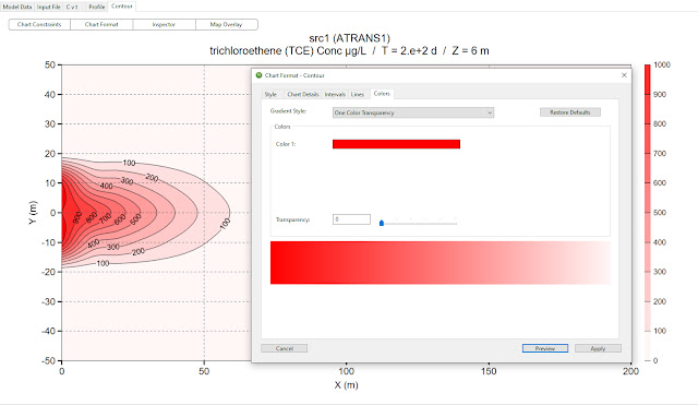
Contour plots in TS-CHEM just got more colorful! In v2023-1 a color spectrum control has been added for contour charts. This allows the user to fine-tune their color scale with up to five colored contour intervals!

In addition to allowing for custom-colored contour intervals, if the user wants to define their concentrations as “high” or “low”, just adjust the Gradient Style to Two Colors and refine the plot.

The new version of TS-CHEM can even represent a single color in style! With the One Color Transparency option the concentrations become more transparent the lower they get, emphasizing where the high concentrations occur in your plume.

Transparency is not just limited to the one-color setting, either! As seen in the figures above, uniform transparency can be applied to the contour plots using any of the color spectrums the user defines. This can be especially useful when combined with the Map Overlay feature!

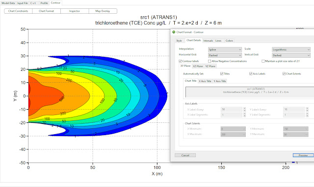
PUT A LIMIT ON YOUR LOG PLOTS

The logarithmic scale (“log” scale) is an important and useful tool when visualizing contaminant plume data. It allows for large differences in concentration to be expressed in an understandable way. For instance, here is a contour plot of a contaminant plume with a linear scale:

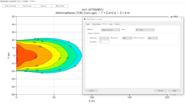
We can see that our concentrations go from 100 – 1000 ug/L, with contours every 100 feet. What if we wanted to see what was going on with the lower concentrations less than 100 ug/L? We can either add a lot more contours or use a logarithmic scale:

We can now easily see our concentrations ranging from 1 to 1000 ug/L with only 10 contour lines. And, in TS-CHEM v2023-1, we can now add a boundary to this log scale plot. For example, we are interested in what the plume looks like between 10 and 1000 ug/L. We can set a plume boundary equal to 10 ug/L and update our plot to reflect this new data range:

These new contour plot controls provide additional tools that can assist the user in producing customized report- or presentation-ready graphics from your TS-CHEM plume transport modeling analyses.

To learn more about the new features of TS-CHEM v2023-1, or to download a FREE DEMO VERSION of the software, visit the TS-CHEM Website today!

State and Federal Guidance Spotlight - Use of TS-CHEM for Estimation of NJDEP Classification Exception Areas

 Introduction

There are a number of state and federal regulatory documents that prescribe the use of solute transport models to support site investigation and remediation activities, along with guidelines on the types of analyses that need to be performed, models that should be utilized, and in some instances, specific input parameters that must be incorporated into analyses. Common applications of solute transport models in state and federal guidance documents include analyses to estimate the expected extent and duration of groundwater plumes, whether sensitive receptors may be impacted, and as a line of evidence to support Monitored Natural Attenuation (MNA) evaluations.  In this first post in the “State and Federal Guidance Spotlight” series, we take a look at the New Jersey Department of Environmental Protection’s (NJDEP’s) Classification Exception Area Guidance, and how TS-CHEM can be used to estimate plume extent and duration to support the delineation of Classification Exception Areas for sites where impacts to groundwater may be present.

Overview of NJDEP CEA Guidance

In the state of New Jersey, groundwaters of the state are classified according to a combination of natural characteristics and actual or potential uses, and groundwater quality standards (GWQS) have been established for these classification areas to ensure that the characteristics and/or actual and potential uses are protected. In instances where GWQS may not be met in a particular area (e.g., an area where impacted groundwater may be present as a result of a discharge of contaminants into the subsurface), the NJDEP requires the establishment of a Classification Exception Area (CEA), which provides notice that the constituent standards for a given aquifer classification are not (or will not) be met over a particular localized area, and that designated aquifer uses in the affected area are suspended for the duration of CEA term.   

CEAs have three main components, including 1) delineation of the horizontal and vertical boundaries of the affected exception area; 2) identification of all groundwater constituents of concern (COCs) to which the exception applies; and 3) an estimate of the longevity of the CEA (i.e., the duration in which COCs will remain above GWQS within the exception area). In the event that the designated use of groundwater within the CEA includes potable use, the NJDEP will identify the CEA as a Well Restriction Area (WRA), which functions as an institutional control by which potable use restriction can be effected (though the NJDEP will not typically prohibit the installation of wells in WRAs).

Appendix A of the NJDEP CEA Guidance provides an overview of the methods that may be used for CEA delineation, and in particular, how to estimate the amount of time required for COCs to reach the GWQS, and the distance in which COCs are anticipated to migrate. With regard to the latter, as long as a sufficient amount of sampling data have been collected, the NJDEP recommends that a “best-fit” methodology to estimate COC attenuation rates (such as the methodology described in the 2003 USEPA issue paper “Calculation and Use of First-Order Rate Constants for Monitored Natural Attenuation Studies”), which can be used to calculate the anticipated time to reach the GWQS.  With regard to the estimation of the maximum distance a plume is expected to travel, the NJDEP identifies several different numerical models that may be used, as well as a more simple analytical solution, which is often utilized by environmental practitioners responsible for the delineation of CEAs at sites in the state of New Jersey.  As discussed in a recent TS-CHEM Blog Post, however,  a 1-dimensional analysis of contaminant transport (such as the one described in Appendix A of the NJDEP CEA Guidance) often greatly overestimates plume extent, resulting in an overly-conservative assessment.  Fortunately, TS-CHEM provides a library of analytical and semi-analytical solute transport modeling solutions that can be used to estimate both the length and duration of groundwater plumes more accurately, without the steep learning curve typically associated with more sophisticated numerical models.

CEA Delineation Using TS-CHEM

As noted above, TS-CHEM, with a library of more than 30 analytical solutions, is perfectly suited to analyze the length and duration of groundwater plumes to assist with CEA development.  The library of solutions allows for the selection of model that is best suited to conditions at a particular site.  For example, at a site where source concentrations appear to be attenuating exponentially, a model like BIOSCREEN-AT may be a good fit.  Or, if source concentrations are variable over time (e.g., as a result of site remediation activities), a model like ATRANS4 may provide the best solution.  And since these models are semi-analytical solutions that analyze the transport of COCs in three dimensions, they are not overly conservative, and as such, will not result in an estimated plume length (and CEA delineation) that is much larger than it is realistically likely to be.

In addition to allowing for the selection of a model solution that best fits conditions at a site, TS-CHEM’s built-in charting and mapping tools can be used to generate all of the necessary output for documenting your analyses (as required when submitting a CEA application), including:

• Charts showing concentration vs. distance and concentration vs. time
• Plots showing plume extents through time
• Mapping tools that allow for the overlay on an interactive digital map of the maximum plume extent in the direction of groundwater flow; or the mapping of plume extent through time to support an application at some point in time for a reduction of the CEA area

Figure 1 - Use of TS-CHEM mapping tool to overlay depiction of maximum plume extent in the direction of groundwater flow

To learn more about TS-CHEM and how it can be used to assist with the estimation of the extent and duration of contaminant plumes, or to download a FREE DEMO of the software, visit the TS-CHEM Website today!

TS-CHEM Example Applications – Receptor Impact Assessment

TS-CHEM is not only simple and easy to use, but it can be applied to a number of different common  situations when it comes to impacted  groundwater, making it the perfect tool for environmental professionals who perform groundwater investigation and remediation activities. To show how TS-CHEM can be used to evaluate a number of common groundwater issues, we have created a series of Example Applications.  In this blog post, we introduce the first Example Application in the series, which demonstrates how TS-CHEM can be used to model the length of a contaminant plume (in this case a benzene plume) in order to determine if it will impact domestic wells at a nearby residential development. You can download the model files and accompanying overview slide deck for the example application described below HERE.

 

Overview

In Example Application 1, there has been a small leak beneath a dispenser island at a gasoline station. This leak has led to a release of benzene into the groundwater below the site with the source concentrated near monitoring well MW-4. A residential development is located 1200 ft (1/4 mile) away from the leak location, and there is concern as to whether domestic wells may be impacted by benzene.  TS-CHEM can be utilized to determine whether the dissolved benzene plume from the dispenser release will reach the domestic wells above the drinking water standard of 5 ug/L.

Fig 1. Site map showing the distance from the benzene source at the dispenser island to the residential area. 

Setting up The Model

Considering the benzene release recently occurred and no remediation has taken place yet, we want to treat the contamination source as constant source rather than a decaying or transient source. Therefore, ATRANS1 is the perfect model solution for this scenario since it is a continuous and constant source model, and it will allow for a conservative evaluation of the maximum extent of the benzene plume.

Once we’ve chosen ATRANS1 as our model solution, we need to input all of the necessary model parameters that have been measured or estimated from a preliminary investigation of the station, as shown below:

• Hydraulic gradient = 0.003 ft/ft
• Hydraulic conductivity = 60 ft/d
• Effective porosity = 0.25
• Benzene source concentration = 3,000 ug/L
• Source width (width of dispenser island) = 10 ft
• Source depth (smear zone thickness beneath water table) = 2 ft

 

Analysis 1

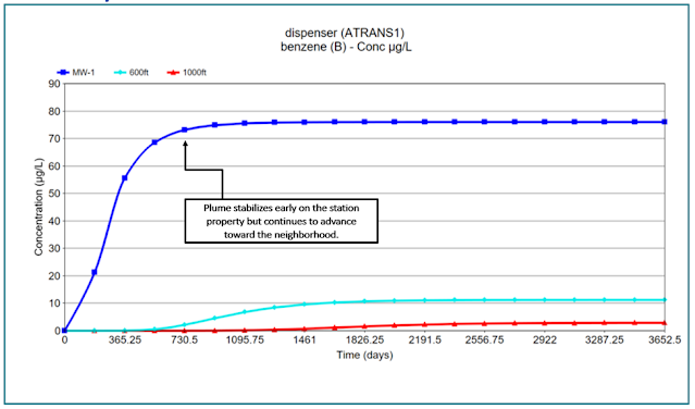
First, we set two model observation points downgradient from the source at 600 ft and 1000 ft away. This will allow us to view the rise and stabilization of the benzene plume at these locations. Next, we run the model for a duration of 10 years. Once the model is finished running, we can display the concentration versus time (C v t) chart:

Fig 2. The C v t chart in TS-CHEM displaying benzene concentrations near the source at MW-1 (dark blue), 600 ft from the source (aqua), and 1000 ft from the source (red).

The dark blue line shows that benzene concentrations at MW-1 where groundwater leaves the station property stabilize at around 76 ug/L, while our observation points we set at 600 ft and 1000 ft show benzene concentrations stabilizing around 11 ug/L and 3 ug/L, respectively. This chart shows how the stabilized concentration of benzene decreases as you move further away from the gas station.

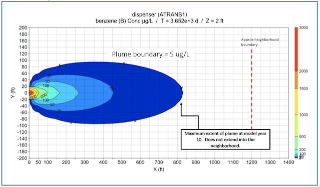
Now, let’s take a look at our contour chart set to model year 10:

Fig 3. TS-CHEM’s contour chart indicates that the maximum plume extent (bound at 5 ug/L) does not reach the residential area.

In the chart above, we’ve set the plume boundary to 5 ug/L, which in this example, is the applicable drinking water standard for benzene. Notice how the maximum extent of the plume does not reach the neighborhood under these model conditions. In this case, one might conclude that based on the results of the analysis, the benzene contamination at the gas station does not impact receptors (domestic wells).

Analysis 2

As noted above, the initial analyses performed using ATRANS 1 indicate that groundwater concentrations are not likely to reach downgradient receptor wells above 5 ug/L. However, let’s say that local regulations impose a different standard, and we must now evaluate a drinking water standard for benzene of 1 ug/L. Accordingly, we will need to perform an additional analysis to evaluate whether downgradient receptor wells may be impacted at concentrations above 1 ug/L.

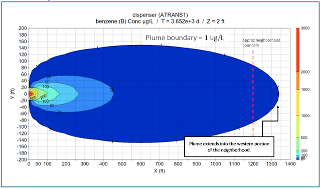
Since nothing at our site has changed (including aquifer characteristics, source concentrations, and source size), we just have to adjust our outer plume contour from 5 ug/L to 1 ug/L. Once we’ve changed the plume contour, we can re-examine the contour chart at model year ten:

Fig 4. TS-CHEM’s contour chart indicates that the benzene plume, with a boundary of 1 ug/L, will impact the residential area.

As shown in Figure 4 above, the plume visibly extends much further to the east than it did in Analysis 1 (Figure 3), and therefore, our conclusion has changed; under this more stringent drinking water standard, the benzene spill at the gas station may impact downgradient receptors. But as noted above, these analyses are very conservative.  What if more reasonable inputs are used?

Analysis 3

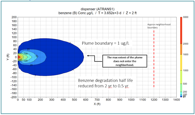
Oftentimes, regulatory agencies prescribe longer half lives for constituents for the purposes of risk evaluations. In many cases, however, half-lives of contaminants like benzene are shorter than the default degradation rates typically prescribed by regulatory agencies. In our last two analyses, we used the default degradation rate of 9.58E-04 d^-1 (half life = 2 years). Let’s change the degradation rate to a more realistic value of 3.8E-03 d^-1 (half life = 0.5 years). After running the model again, there is a noticeable difference in the concentration and length of the benzene plume.

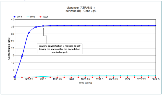
Fig 5. The C v t chart in TS-CHEM shows that benzene concentrations stabilize at a much lower level when the degradation rate is increased.

As shown in Figure 5 above, the C v t chart shows that benzene stabilizes around 35 ug/L at MW-1 near the station property boundary, which is about half the concentration observed in the previous analyses. Additionally, the benzene barely registers at our downgradient observation points. Now let’s look at the contour chart to examine the maximum extent of the plume using this higher degradation rate.

Fig 6. The contour chart demonstrates the effect of increasing the degradation rate of benzene. The plume, while still bound at the more protective 1 ug/L, no longer impacts the residential area.

Review of contour charts for each model year indicates that the benzene plume stabilizes in less than 4 years, which is about half the time it took the plume to stabilize in the previous analyses. Also, the plume, bound at 1 ug/L, reaches a maximum length of approximately 580 ft, and thus, does not impact the neighborhood domestic wells. The length of the benzene plume observed in this analysis is consistent with benzene plume lengths seen in many literature studies such as API 1998 and Connor et al 2014.

Why is this important?

In the case of a leak or spill of hazardous substances, government agencies may require some form of receptor impact evaluation in order to protect people and ecological receptors from exposure to contamination. TS-CHEM is a quick and easy, and science-base, way for any environmental professional to assess potential risks to receptors, evaluate the effect of changes in input parameters, and support decisions regarding the possible need for remedial actions. With over 30 solution models to choose from and a library of the most commonly modeled constituents, you can select an appropriate model and quickly (and easily) perform a receptor impact evaluation at your site!

To learn more about TS-CHEM, or to download a FREE DEMO of the software, visit the TS-CHEM Website! If you would like to see what else TS-CHEM can do, check out our other Example Applications!