New Plume Center of Mass Analysis Tool

Introduction

Groundwater contaminant plume remedy plans that are considering Monitored Natural Attenuation {MNA} are often required to demonstrate a stable plume. i.e. they must provide data or an analysis to verify that the plume is no longer advancing downgradient from the source area toward potential receptor locations.

One method to graphically depict plume stability involves determining the center of mass of the plume over some period of time.

 

Previous Guidance and Methods

In 2000, the Air Force Center for Environmental Excellence (AFCEE) published MNA guidelines (Wiedemeier et al. 2000) that described methods for evaluating the feasibility of an MNA remedy. Tracking plume center of mass to determine plume stability was cited as one of the primary methods.

In 2008, Ricker published methods for evaluating stability of a groundwater plume. For one of the methods, Ricker included a formula for calculating plume center of mass in two dimensions (Ricker 2008).

In 2022, New Jersey Department of Environmental Protection (NJDEP) issued MNA guidance that discussed methods for performing spatial analysis of trends in contaminant plume mass. In particular, the guidance cites to Ricker’s methods and to the AFCEE 2000 guidance center of mass analysis.

In 2024, Golden Software published information on its website describing the use of its Surfer spatial analysis software to apply the Ricker method to contaminant plume center-of-mass analysis.

It is clear from this history that regulatory guidance and industry practice has highlighted the need for a method, or methods, to demonstrate that a groundwater contaminant plume is stable when considering MNA as a part of the overall remedy.

 

TS-CHEM Center of Mass Analysis Tool

Building on the previously identified usefulness of software tools for demonstrating plume center-of-mass stability, the latest version of TS-CHEM - - v2024-3 released in June 2024 - - includes a new Analysis Tool that is capable of calculating the center of mass for any plume, or set of commingled plumes, generated by the software.

 

As an example, a simple benzene plume transport model was developed and run for 10 years, with output every 2 years. 

The TS-CHEM Plume Center of Mass analysis tool operated on the model output shown above to generate data depicted in the figure below.

The output calculated by the TS-CHEM Center of Mass Analysis Tool demonstrates that the benzene plume center of mass location relative to the source (X distance from the source) stabilizes at a time about 7 years after the initial benzene release.

 

Conclusion

One of the key analyses that can prove beneficial in supporting a Monitored Natural Attenuation remedy is a demonstration that the plume is stable in time, which can be verified by demonstrating that the location of the plume center of mass has stabilized. This concept, as well as several methods of making this demonstration, are described in regulatory guidance and in the scientific literature.

 

TS-CHEM has recently incorporated a method similar to the Ricker 2008 center of mass method as one of its built-in analysis tools. In the simple example shown above, the analysis demonstrates that the plume is in a stable configuration after about 7 years, which could support consideration of Monitored Natural Attenuation as a feasible remedy.

 

References

Golden Software 2024. The Ricker Method for Plume Stability Analysis. Golden Software website:

https://www.goldensoftware.com/ricker-method-for-plume-stability-analysis/

 

NJDEP 2022. Monitored Natural Attenuation Technical Guidance. Contaminated Site Remediation & Redevelopment Program, 178 pp; Appendix F – Selected Reference Summaries.

 

Ricker, JA 2008. A practical method to evaluate ground water contaminant plume stability. Ground Water Monitoring & Remediation, 28(4), p. 85 – 94.

 

Wiedemeier, TH, MA Lucas, and PE Haas 2000. Designing Monitoring Programs to Effectively Evaluate the Performance of Natural Attenuation. Air Force Center for Environmental Excellence, 55 pp.

Simplify Source Model Set-Up with the New CSV Import Feature

One exciting addition in the latest release of TS-CHEM (version 2024-3) is the new “CSV Import” feature for time-varying source concentrations. Several of the TS-CHEM solutions allow the user to specify source concentrations that change with time (ATRANS3 and ATRANS4; AT123D-AT FT and AT123D-FT). The gradually varying concentration being released from the actual source (smooth red curve in the chart below), is represented in the TS-CHEM analytical model as a series of concentration steps (blue step changes in the chart below).

The CSV Import feature can be used to efficiently set up and solve a time-varying source model by allowing users to import time-and-concentration source histories that have been created manually by the user, or exported from other user software, in CSV format. For example, the SILT soil source leaching model is capable of calculating and exporting a CSV file of groundwater source concentrations from a soil zone contaminant source (see the SILT Blog Post for more information).  

User-created source history files can be used to analyze various scenarios for releases from an industrial facility over time. Concentration versus time output from software that calculates source release concentrations - - for example, SILT leaching a contaminant from soil to groundwater or SourceDK representing dissolution and dissipation of a NAPL source - -  can be saved as a CSV file and imported directly into TS-CHEM.

Using the new CSV Import feature is simple. In the Model Data tab, for transient (stepped through time) concentration data sets, begin by clicking in the data entry field, and a data entry pane is opened on the right side of the window to facilitate data entry (see Figure 1).

Figure 1. Source Concentration Data Entry Pane

To import a time-and-concentration source history file (in CSV format), click on the Import button to open the CSV data import control panel (see Figure 2).

Figure 2. Import CSV Data List Window

Click on the Choose button and navigate to the CSV data file. The file contents will be displayed in the Preview window. Use the “Significant Digits” setting to format the concentration values to improve viewability (excessively long concentration values with many digits to the right or left of the decimal point can be difficult to read). If the file was created with a header row, the check box can be used to eliminate that row before import.

Checking the “Replace” check box will completely replace (overwrite) all data pairs currently in the source history list. Unchecking the “Replace” check box will merge the CSV file data pairs into the current source history list, and will sort the list to properly organize the specified history of concentrations. Note: If there is a time-and-concentration data pair in the CSV file with a time identical (within 1E-04) to a time already in the source history list, the CSV file data pair will overwrite the current list data pair; thereby effectively specifying an updated concentration for that time.

Click the Import button and the CSV file data will be added to the source history list (see Figure 3).

Figure 3. Source Concentration Data Entry Pane (with imported data)

In addition to the new CSV Import feature, several other updates and improvements have been incorporated into TS-CHEM version 2024-3, including:

• Plume Center of Mass analysis tool for MNA and other analyses
• Data entry enhancements
• Other minor improvements and bug fixes

To take advantage of these updates and improvements and test out the new CSV Import feature, head over to the TS-CHEM Website to download version 2024-3 today!

Supplemental TS-CHEM Installation Instructions for Mac Users

Currently, TS-CHEM is an Intel-based application, and as a result, certain Apple products (MacBook Pro, MacBook Air, iMac, Mac Mini, etc.) that contain Apple silicon chips (e.g., M1, M2, or M3) may not be able to solve TS-CHEM models, producing a message in the run window noting that there is a “Bad CPU type in executable” (see example below).

To solve TS-CHEM models on Apple Macintosh computers that contain Apple chips, users can install the Rosetta 2 software*, which allows those machines to run Intel-based applications.  To install the Rosetta 2 software, follow the steps below:

    1.    Open up the Terminal application

    2.    Copy and paste the following text in the command prompt:

                softwareupdate --install-rosetta

    3.    Press Enter, and follow the subsequent prompts to install the software.

Once the Rosetta 2 software is successfully installed, machines with Apple chips should be able to run TS-CHEM models without any issues.  

Please contact the TS-CHEM Support Team (Support@TS-CHEM.com) if you have any questions, or if you require any assistance with installing the Rosetta 2 software.

*Rosetta is an Apple utility that enables a Mac with an Apple silicon CPU to use apps built for a Mac with an Intel processor. (see https://support.apple.com/en-us/102527). Computers in this category are listed on the Mac computers with Apple silicon web page (https://support.apple.com/en-us/116943).

 

New Modeling Tools – SCL Plume Model and PVM Calculator

The TS-CHEM team is pleased to announce the release of two new Microsoft Excel-based spreadsheet utilities – the SCL Plume Model, and the Plume Volume and Mass (PVM) Calculator.  With straightforward inputs and intuitive numeric and graphic outputs, these tools allow environmental practitioners to quickly estimate the extent of plumes at specified points in time, and get a sense of key plume characteristics, including the volume of impacted groundwater within the contaminant plume, the mass contained within the plume, and/or the mass flux across a user-specified plume transect.

SCL Plume Model Spreadsheet

Since the mid-1980s, one of the most widely used analytical plume transport models has been what is generally referred to as the Domenico model. The Domenico model has been applied by regulatory agencies as the basis for a number of software tools (e.g., USEPA’s BIOSCREEN and BIOCHLOR; CA RWQCB spreadsheet; PADEP Quick Domenico spreadsheet), and has been widely applied and reported on in the professional and scientific literature.  Beginning in approximately 2005, investigators began commenting on perceived inaccuracies in the approximate Domenico solution, and in 2007, an improved solution that maintains the efficiency of the Domenico solution, and reportedly improves on its performance was developed and published by Srinivasan et al. (2007).  That efficient solution has been programmed into the SCL Plume Model spreadsheet, which can quickly generate calculated data outputs and model results charts that can assist practitioners in examining and better understanding plume behavior at their site of interest.

Input data for the SCL Plume Model include the common parameters required for an analytical plume transport model, including:

• source information (source dimensions and source concentration);
• aquifer parameters (hydraulic conductivity, horizontal hydraulic gradient, and effective porosity);
• contaminant transport parameters (dispersion, retardation rate, and degradation rate);
• time information (time at which source concentrations are to be calculated); and
• plot parameters (several inputs that control numeric and graphic model outputs).

Users can also specify a groundwater standard (which allows the user to examine where the plume concentration along the centerline drops below the specified concentration) as well as the distance to the nearest receptor (which allows the user to examine the model estimated constituent concentration at the receptor location).

The SCL Plume Model spreadsheet generates calculated data outputs (including concentrations along the plume centerline at a specified point in time) and model results charts (including a concentration vs. distance chart and plume contour chart).  

Figure 1. SCL Plume Model spreadsheet interface, including model input tables, plume centerline chart, and plume contour chart

Plume Volume and Mass (PVM) Calculator Spreadsheet

The slow dissolution of a chemical of concern (COC) from a subsurface waste zone or spill through soil into slowly seeping groundwater can form a sizeable area of downgradient contamination above some water quality standard (e.g. maximum contaminant level MCL), frequently referred to as a plume. It is often helpful in an environmental site investigation to develop certain metrics that describe properties of the groundwater plume to aid in forming a more quantitative conceptual site model.  The Plume Volume and Mas (PVM) Calculator is designed as a Microsoft Excel spreadsheet-based tool that can assist site investigators with estimating key plume metrics, allowing them to easily input parameters describing the geometry of the plume as it has been mapped in the field, and then to calculate a variety of outputs, including:

• Areal extent and overall volume within the aquifer that is occupied by the plume;
• Volume of contaminated groundwater within the aquifer pore space;
• Mass of dissolved and sorbed chemical of concern in certain concentration contour zones of the aquifer;
• Overall mass of chemical in the plume; and,
• Mass flux across a user-specified transect.

The basic concept underlying the method applied in this tool is that, because of the nature of most groundwater plumes, their overall shape, as well as the shape of the various nested concentration contour zones, can be represented fairly well by a set of nested ellipsoid-shaped volumes (see Figures 2 and 3 below).

Figure 2. Diagram of a typical groundwater contaminant plume (plan view) mapped from a horizontally spaced array of monitoring wells.

Figure 3. Diagram of a typical groundwater contaminant plume (cross-section view) mapped from vertically spaced monitoring wells (e.g. shallow, intermediate, and deep intervals).

The “field mapped” plan view and cross-sectional plume diagrams generated by the environmental investigator are used as the basis for measuring the ellipse dimensions (i.e., the length, width, and thickness for each isoconcentration contour) that form the required set of nested ellipsoid data to be input into the PVM Calculator.

Figure 4. Nested ellipsoids calculated by the PVM Calculator based on user-specified inputs.

In addition to entering estimated dimensions for each plume isoconcentration contour interval, the user can also specify parameters for the constituent of concern (including the name of the chemical and its associated density) and aquifer properties (including hydraulic conductivity, horizontal hydraulic gradient, and effective porosity).  The user can also specify a location along the plume at which mass flux is calculated through a vertical plane (i.e., YZ plane) that is oriented perpendicular to the X direction of groundwater flow.

Based on the user-specified inputs provided, the PVM Calculator estimates the following for each isoconcentration contour interval:

• area
• volume
• dissolved and sorbed chemical mass
• chemical volume

Additionally, the PVM Calculator also estimates the contaminant mass flux across a vertical plane transect (if specified by the user).

These plume metrics are useful for a variety of conceptual site model development and remedy planning project steps.

The SCL Plume Model and PVM Calculator spreadsheet each include a detailed User Guide which provides a comprehensive overview of the tools, step-by-step instructions for all inputs, descriptions of the calculations that are performed, and references to literature on which the tools are based. And, the tools are available FREE of charge on the TS-CHEM website.

To learn more about the SCL Plume Model spreadsheet, or to download a copy, click HERE.  To learn more about the PVM Calculator spreadsheet, or to download a copy, click HERE.

Estimation of TS-CHEM Source Terms Using the Newly Released Soil Infiltration and Leaching Tool (SILT)

TS-CHEM is pleased to announce the release of the “Soil Infiltration and Leaching Tool” (SILT), a  Microsoft Excel-based spreadsheet utility that allows users to simulate one-dimensional contaminant fate and transport processes though the vadose zone in a simple, user-friendly environment.  The SILT utility is a perfect companion to TS-CHEM, allowing site investigators to evaluate potential impacts to groundwater associated with contaminated soil, and estimate contaminant source terms that can then be incorporated into TS-CHEM and used to estimate the extent and duration of resulting contaminant plumes.  

Figure 1: Vadose Zone Transport Conceptual Model for SILT

SILT simulates contaminant transport from the soil source, through the vadose zone, to a groundwater contaminant source zone in three basic steps:

1.  The initial source zone water concentration, located in the Source Zone (of user-specified vertical thickness), is calculated after partitioning of the user-specified Source Zone Total Soil concentration among the solid-, air- and dissolved phases

2.  The dissolved phase contaminant source is transported vertically downward through the Vadose Zone, being acted upon by dispersion and degradation processes, until it reaches the  groundwater table, producing a leachate breakthrough curve

3.  At the bottom of the vadose zone, leachate (at the calculated flux rate and concentration) is delivered to a mixing zone at the top of the water table. When the infiltrating soil water reaches the water table, it is mixed with groundwater and the contaminant is diluted (using a Dilution Attenuation Factor (DAF)), resulting in a lower concentration. The diluted concentration data can then be used for comparison to published groundwater standards, and/or utilized to calculate source terms for groundwater plume models (such as TS-CHEM).

Figure 2: Groundwater Source Term Conceptual Model for SILT.

SILT’s Interface is set up in an intuitive manner, with a series of worksheets that allow for a streamlined, step-by-step workflow.  These worksheets are described below.

•  Step 1 – Source Zone – In this worksheet, the user can specify fate and transport parameters for the contaminant of concern in the soil source zone, as well as the amount of time soil leachate concentrations will be calculated for, and the nature of the source (e.g., constant source, decaying source, or variable source concentrations), allowing the user to estimate soil source concentrations through time.

Figure 3: Source Concentration Input Table in SILT “Source Zone” tab.

•       Steps 2 and 3 – Vadose Zone and Mixing Zone – Using the soil source zone concentrations estimated in Step 1, the Vadose Zone and Mixing Zone worksheet allows the user to input properties of the vadose zone soils (e.g., distance from bottom of source to water table, water content, and seepage velocity) and the contaminant as it migrates downward through the vadose zone (e.g., decay rates in water and soil) to estimate leachate concentrations at the bottom of the soil column.

Figure 4: Worksheet layout for the “2 Vadose & 3 MixingZone” Tab – Step 2

      The leachate concentrations estimated as part of Step 2, along with a DAF value (which can be specified by the user or calculated using multiple methods) are then used to estimate dissolved-phase concentrations in mixing zone groundwater beneath the soil source zone.

 

Figure 5: Worksheet layout for the “2 Vadose & 3 MixingZone” Tab – Step 3

• Step 4 – Plume Model Source Steps – In this worksheet, the user can discretize the diluted mixing zone groundwater concentration data estimated in Step 3 into a specific number of source concentration steps (each with its own duration), which can then be incorporated into a groundwater contaminant plume model (such as TS-CHEM) as a source term.

Figure 6: Worksheet layout for the 4 Plume Source Steps Tab.

SILT also incorporates a number of features that facilitate model input, and allow for easy export of model results.  For example, SILT includes a “unit conversion” feature, which allows the user to enter a variety of commonly used units for most input parameters, which are automatically converted by the model before running model calculations. This feature prevents unnecessary confusion related to units and ensures model output is consistent and accurate, while also allowing greater flexibility.  Additionally, users can export time series charts of model output with the click of a button (including modeled source concentrations, leachate concentrations, diluted groundwater concentrations in the mixing zone, and plume model source steps). Model generated time step source concentrations can also be exported to a comma-delimited .csv file, allowing for easy incorporation into groundwater plume models as a source term.

SILT includes a detailed User Guide which provides a comprehensive overview of the SILT utility, step-by-step instructions for all model inputs, and thorough descriptions of the calculations that are performed in SILT. And, if you’re not sure where to start, SILT comes packaged with a built-in example soil leaching model that simulates migration of TCE through the vadose zone, and is based on vadose zone fate and transport parameters presented in Sanders (1995). Simply click the “Sanders 1995 Example Model” button on the “1 Source Zone” tab, and all associated input parameters will be populated in the model worksheets. 

The SILT utility can be downloaded for FREE from the TS-CHEM website (https://www.transportstudio.com/SILT/).

TS-CHEM Example Applications – Commingled Plume Analysis

In the course of performing site investigations, environmental professionals are often tasked with identifying sources of contamination (e.g., areas where contaminants may have been discharged into site soils and may have potentially migrated to groundwater) and delineating the nature and extent of impacted groundwater. In many cases, releases of the same chemical from multiple operational area sources may form downgradient plume zones that commingle, making it difficult to distinguish which source (or sources) may be responsible for impacted groundwater. Additionally, commingling of a site groundwater plume (or plumes) with plumes from off-site sources may further complicate the determination of source contribution and responsibility for cleanup. 

Although evaluating which source (or sources) of contamination at a site (or sites) may be associated with impacted groundwater when commingled plume conditions are present can be difficult, there are resources and tools that can assist environmental professionals with demonstrating that commingled plumes are present and assessing the relative contribution from individual plumes to the commingled plume. For example, New Jersey’s Commingled Plume Technical Guidance Document (which can be accessed HERE) describes several types of commingled plume scenarios that may be encountered, how to investigate them, and how to develop lines of evidence to evaluate commingled plume conditions and select appropriate remedial measures. 

One of the lines of evidence identified in the New Jersey Commingled Plume Guidance Document is solute transport modeling. With TS-CHEM, site investigators can quickly and easily perform solute transport modeling analyses to evaluate commingled plume conditions at a site and establish a clear line of evidence that demonstrates likely contribution from each source area identified, and which plume(s) may contribute to known and potential impacts to downgradient receptors. 

This blog post will cover the fourth Example Application in the TS-CHEM Example Application series: Commingled Plume Analysis. To follow along and review the model files, you can download this example application HERE.

Overview

In this scenario, investigators have identified areas of concern associated with historical releases of chlorinated solvents from degreasers at two separate nearby industrial sites, resulting in the release of Trichloroethylene (TCE) to groundwater. The plumes associated with these releases have apparently commingled, resulting in a plume that extends downgradient from the sites. A well search has identified a potential receptor well 3,000 feet downgradient from one of the sites. Initial site investigations have revealed the following information:

• Aquifer material = medium sand; some gravel; little silt
• Hydraulic gradient to the east = 0.003 ft/ft
• Source area TCE concentrations:
• Source 1 = 10,000 µg/L
• Source 2 = 5,000 µg/L

Figure 1. Site map showing source areas, distance to downgradient receptor well.

Concerned by potential impacts to the downgradient receptor, regulators have requested that analyses be performed to determine whether TCE will impact the downgradient receptor well in exceedance of applicable the standard (in this case 5 µg/L), and if so, which site (or sites) may be responsible for impacts to the well.   

Setting Up the Model

The releases of TCE at the two sites have resulted in the identification of Dense Non-Aqueous Phase Liquid (DNAPL) in the subsurface, and as such, the DNAPL source areas at the two sites are located at approximately 16 ft beneath the water table. Because of this, 3DADE-3 is a good model solution for this analysis because it is capable of representing the source areas as a vertical patch source at depth and assumes a constant concentration (which is appropriate since ongoing DNAPL sources are present beneath both sites). In TS-CHEM, the following model parameters should be set

•  Hydraulic gradient = 0.003 ft/t
• Hydraulic conductivity = 80 ft/d
• Effective porosity = 0.25
• Source width = 20 ft
• Source depth = 16 ft
• Source Thickness = 4 ft
• Source 1 TCE source concentration = 10,000 µg/L
• Source 1 TCE source concentration = 5,000 µg/L

Analysis 1: Assessing Potential TCE Impacts to Downgradient Receptor Well

First, a model observation point should be set approximately 3,000 ft downgradient from Source 1 (i.e., the location of the receptor well). After running the model for approximately 40 years, the C v t plot reveals that the commingled plume first reaches the receptor well after 10 years and stabilizes after approximately 28 years (when concentrations begin to level off just above 30 µg/L) (Figure 2).

 

Figure 2. The C v t chart in TS-CHEM displaying commingled plume TCE concentrations at the receptor well (located 3,000 ft downgradient from Source 1).

Although this analysis answers the question as to whether the commingled plume may impact the downgradient receptor well in exceedance of the applicable standard of 5 µg/L for TCE (it will), we also want to understand the extent to which each of the source areas may contribute to those impacts (including which source/plume first reaches the well, and the extent that each well contributes to TCE impacts). This analysis can easily be done in TS-CHEM by simply unchecking the “sum concentrations” option, which will display individual contributions from each plume on the C v t plot.

Figure 3. The C v t chart in TS-CHEM displaying TCE concentrations associated with plumes from Source 1 and Source 2  at the receptor well (located 3,000 ft downgradient from Source 1).

As shown in Figure 3, although the plume associated with Source Area 2 is the first to reach the receptor well, with the plume from Source Area 1 arriving soon after.  The plot also indicates that after about 20 years, Source Area 1 is contributing about 2/3 of the TCE in the receptor well, whereas the plume associated with Source Area 1 is contributing approximately 1/3 of the TCE (once the plumes stabilize).

TS-CHEM also allows for the generation of contour plots, which in this case, indicate that the plumes from the two source areas begin to commingle after approximately two years (Figure 4), with the commingled plume reaching a maximum extent of approximately 4,000 ft after 20 years (Figure 5).

Figure 4. TS-CHEM's contour chart showing initial commingling of plumes after two years

Figure 5. TS-CHEM's contour chart showing extent of commingled plume after 20 years

Analysis 2: Evaluation of Potential TCE Impacts to Downgradient Stream 

As shown in Figure 1, there is a stream located approximately 5,000 ft downgradient from Source Area 1, and regulators have expressed some concern as to whether the stream may be impacted by one or both of the TCE plumes above the standard 5 µg/L.  To examine this, we can add an observation point in the location of the stream (i.e., 5,000 ft downgradient from Source 1), and then examine the C v t plot.  As shown in Figure 6, the commingled plume reaches the stream after approximately 22 years and exceeds the applicable cleanup standard (5 µg/L) after approximately 30 years.  But, when we examine individual plume contributions, we can see that although the plume associated with Source Area 2 reaches the stream first, the concentrations associated with that plume do not exceed the applicable cleanup standard, whereas the TCE concentrations from Source Area 1 plume do exceed the standard (Figure 7).

Figure 6. The C v t chart in TS-CHEM displaying commingled plume TCE concentrations at the stream (located 5,000 ft downgradient from Source 1).

Figure 7. The C v t chart in TS-CHEM displaying TCE concentrations associated with plumes from Source 1 and Source 2  at the stream (located 5,000 ft downgradient from Source 1).

Analysis 3: Examining A Higher Plume Degradation Rate

Oftentimes, regulatory agencies prescribe longer half-lives for constituents for the purposes of risk evaluations. In many cases, however, half-lives of contaminants like TCE may be shorter than the default degradation rates typically prescribed by regulatory agencies. In the analyses performed thus far, a TCE half-life of 10 years was assumed.  For this analysis, we want to examine TCE impacts at both the receptor well and the stream if the TCE half-life of the plume is shortened to 4.5 years.

Figure 8. TS-CHEM's contour chart showing extent of commingled plume with shorter TCE half-life after 20 years.

The contour chart shown in Figure 8 indicates that after 20 years, the commingled plume boundary is reduced by approximately 500 ft when compared to Analysis 1 when the TCE half-life is reduced to 4.5 years. As shown in the C v t plot in Figure 9, although the commingled plume TCE concentration still exceed the applicable standard of 5 µg/L at the receptor well, concentrations do not exceed the standard at the downgradient stream.  

Figure 9. The C v t chart in TS-CHEM displaying TCE concentrations associated with plumes from Source 1 and Source 2 at the receptor well and stream (assuming a 4.5-year TCE half-life).

Conclusion

The presence of commingled plume conditions at sites can be challenging for environmental professionals responsible for investigating and remediating impacted groundwater, making it difficult to determine the extent to which sources may contributing to the commingled plume, and in turn, who may be responsible for cleaning them up. In this exercise, we demonstrated how TS-CHEM can be used to perform quick and easy analyses that allow site investigators to not only quantify the impacts of the commingled plume (e.g., impacts to downgradient receptors), but also evaluate the individual contributions from each source. This line of evidence (along with other lines of evidence developed by the site investigator) can be used to determine which party (or parties) may be responsible for impacted groundwater, and in turn, who should pay for the associated investigation and cleanup. 

TS-CHEM Solution Library - AT123D-AT

The TS-CHEM program provides an easy-to-use software environment in which to analyze contaminant plume transport, and includes a comprehensive library of more than 30 different analytical solutions to the advection-dispersion equation. Each solution incorporates different capabilities, including how it represents the contaminant source and how the plume interacts with the aquifer. For this post in the Solution Library series, we will be focusing on the AT123D-AT family of models published by Dan Burnell in 2012 which represents an updated version of the original AT123D model suite developed by G.T. Yeh at the Oak Ridge National Laboratory.

What is AT123D?

The original AT123D was a suite of analytical model solutions that are used to simulate one-, two- and three-dimensional transport in groundwater. The program is complex, and allows for many different source configurations, including

• patch sources
• line sources
• point sources
• volume sources

In contrast to many analytical plume models that represent the source using a first-type specified concentration, AT123D represents the source as a second-type specified mass flux boundary condition. This means, for example, if you know the nitrogen load from a residential dwelling to a septic system (i.e. number of residents times average daily nitrogen load per person) you can represent that source in AT123D as milligrams of nitrogen per day instead of trying to estimate a septic source concentration value. The primary difference between AT123D and AT123D-AT is in how the solver arrives at a solution to the advection-dispersion equation. AT123D-AT incorporates a Romberg numerical integration scheme that works to prevent oscillations, speed convergence, and improve accuracy for a wide range of input parameter combinations.

A conceptualization of the many possible specified mass flux source geometries available in AT123D-AT is shown in Figure 1 below, and can also be found in the Model Selection Tool in TS-CHEM:

Figure 1 - AT123D-AT Source Geometries

TS-CHEM was developed with usability in mind, so the numerous AT123D-AT solutions available to the user (differing aquifer geometries, source geometries, and source types) have been broken up into six “versions” (see table below). These pre-configured versions allow the user to select the type of AT123D-AT model that will best represent their site (aquifer and source), and to specify the desired parameter input values to represent site-specific properties, using model types that closely match conditions simulated by other analytical ADE solutions included in ­TS-CHEM’s Solution Library. This last consideration makes it easier to compare different plume transport solutions (e.g. a first-type source vs a second-type source) by selecting similar type models (e.g. with aquifer boundaries or without aquifer boundaries) from the TS-CHEM Solution Library.

The following nomenclature is used between each version to help the user quickly determine which version they are looking for: Infinite boundary (I), Finite boundary (F), Constant mass release rate (C), Instantaneous release source (I), Time-variable (transient) mass flux (T):

Model Version	Aquifer Boundary	Source Type	Analagous TS-CHEM models
AT123D-AT IC	Infinite unbounded	Constant mass flux	3DADE-3 or 3DADE-4 (patch source)
AT123D-AT II	Infinite unbounded	Initial mass instantaneous release	3DADE-5 or 3DADE-6 (volume source)
AT123D-AT IT	Infinite unbounded	Constant specified concentration	ATRANS4 (with concentration stepping)
AT123D-AT FC	Finite bounded	Constant mass flux	ATRANS1
AT123D-AT FI	Finite bounded	Initial mass instantaneous release	3DADE-5 or 3DADE-6 (volume source)
AT123D-AT FT	Finite bounded	Constant specified concentration	ATRANS4 (with concentration stepping)

What are the differences between the AT123D-AT models?

The two defining factors that highlight the differences between the different AT123D-AT models are 1) whether the aquifer extent is assumed to be infinite (as is the case for many analytical transport solutions) or finite (bounded horizontally or vertically), and 2) how the source concentration or flux is applied at the model boundary over time (continuous, instantaneous pulse release, or time-varying). The three different types of source concentration fluxes are conceptualized in Figure 2 below:

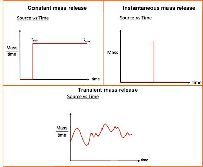
Figure 2 - AT123D-AT Model Source Types

As you can see in Figure 2, there are three distinct source types. The source type that is most appropriate to use in a particular application is dependent on the known conditions at a site, and/or the known or assumed conditions of the source.

What applications are the AT123D models best suited for?

As discussed in previous blog posts, TS-CHEM can assist environmental professionals with the development of conceptual site models (CSMs) that characterize the extent and behavior of groundwater contaminant plumes. The AT123D-AT models are highly flexible, able to provide users with the ability to evaluate solute fate and transport in one-, two- or three-dimensions. In its fundamental form, AT123D-AT is solving the 3D ADE equation in a 1D (X-direction only) aquifer flow field, but 2D plume transport and even 1D “column” transport can be set up using the bounded aquifer settings. i.e. the AT123D-AT “F” models (FC, FI, and FT) can be used to represent sites where the aquifer thickness and/or width is known or is believed to be bounded (finite aquifer boundary). This type of AT123D-AT model is similar to the ATRANS family of models which include an upper (water table) and lower (aquifer base) no-mass-flux boundary.

But the AT123D-AT models are not all limited to bounded aquifer conditions. The AT123D-AT “I” models (FI, II, and IT) can be used to represent sites where there is no limitation on aquifer thickness or width (infinite aquifer boundary). This type of AT123D-AT model is similar to the 3DADE family of models, which do not impose any finite boundaries on the aquifer.

Further, the investigator can use a variety of patch source geometries to best represent the conditions at their site. For example, if an investigator has information on source mass flux at the downgradient edge of a source area, they may use a patch source. Or, if a large regional scale model is being considered, the user may want to utilize a point source to track the general plume behavior over time.

When choosing between source types, a user may choose to use a constant mass release source AT123D-AT model If only a single source concentration is known, and/or the investigator wished to perform a conservative analysis in which the source does not deplete through time. If the user wanted to investigate the plume behavior in a case where a slug of solute is introduced into the groundwater, they can use an instantaneous release source type. If information is available on the changing history (both increases and decreases) of source flux over time, the transient source type can be used.

Similar to the ATRANS1 model, the AT123D-AT FC model is useful for simulating scenarios that have aquifers of a finite extent that can be represented by a continuous mass flux. This type of analysis may be useful for evaluating a conservative maximum plume extent, or when the plume becomes stable (Figure 3):

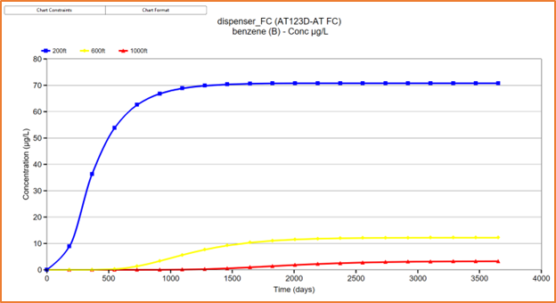
Figure 3 - AT123D-AT FC solution showing maximum plume extent for a stable benzene plume with a constant source flux of 0.001 ld/d at 200ft, 600ft and 1000ft from the source.

The AT123D-AT FI model is useful for simulating scenarios where a slug of contaminant is assumed to have rapidly entered the groundwater. This type of model is sometimes used in an emergency spill response analysis if an investigator wants to simulate a conservative condition where a “slug” of contaminant enters the groundwater instantaneously and then is allowed to flush away from the spill area toward a possible receptor location (Figure 4):

Figure 4 - AT123D-AT FI solution showing plume concentrations up to 4000 days after an instantaneous mass input of 22.05 lbs of benzene introduced to groundwater. Concentrations are shown at 200ft, 600ft and 1000ft from the source. 

Similar to the ATRANS4 model, the AT123D-AT FT model allows the user to define transient source behavior. Unlike ATRANS4, the AT123D-AT FT model uses a second-type boundary condition and is therefore defined by time-flux pairs (instead of time-concentration pairs). The transient source condition allows the user great flexibility in how they define the time series of their source and can enable investigators to simulate complex scenarios where there may be intermittent single sources, multiple sources that overlap at different times, or even source termination that would result from remedial actions.

An example of a time-variable source flux is shown in Figure 5 below for a hypothetical release from an underground storage tank (UST). The benzene source progressively decreases until it eventually reaches zero after 2000 days. This might be indicative of a UST that leaks over time, or it could be indicative of a UST removal at around 500 days with a small amount of product remaining after removal. In either case, the benzene concentration is reduced over time through degradation/natural attenuation and flushing.

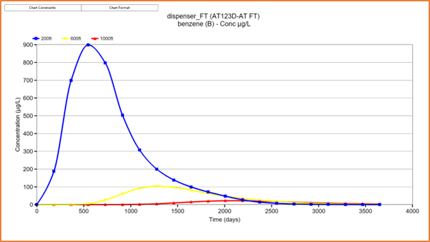
Figure 5 - AT123D-AT FT solution showing benzene plume concentrations entering groundwater from a hypothetical underground storage tank at 200ft, 600ft and 1000ft from the source.

To summarize: the AT123D-AT family of models available in the TS-CHEM Solution Library allow for a very flexible representation of the source over space and through time and can be used for a variety of environmental scenarios and conditions. The feature that sets the AT123D-AT models apart is that they are the only models in the TS-CHEM solution library that utilize a second-type (specified mass flux) source boundary condition, allowing for users to directly input an estimate of source mass flux for their site. AT123D-AT also differs from AT123D in that it incorporates enhanced solver capabilities that reduce solve times and increase solution accuracy. The six AT123D-AT model types included in TS-CHEM allow a user to easily identify which model is best for their site or application. These models can assume either a finite or infinite aquifer boundary and a multitude of source geometries and source release types.

To learn more about TS-CHEM, or to download a FREE DEMO VERSION of the software, visit the TS-CHEM Website today!