TS-CHEM Example Applications – Natural Source Flushing with MNA

 Monitored Natural Attenuation (MNA) is a remediation method that relies on natural processes to decrease contamination in the soil or groundwater. It is a popular method of remediation since it tends to involve less equipment and labor and therefore, less cleanup costs. 

Scientists typically monitor the contamination at a site to ensure that it is attenuating properly and within a reasonable time period. According to New Jersey’s MNA guidance, the applicability of MNA must be demonstrated by lines of evidence directly or indirectly indicate that natural attenuation processes are occurring. With TS-CHEM, it is simple to establish a clear line of evidence that demonstrates natural attenuation is occurring at your site.

This blog post will cover the second Example Application in the TS-CHEM Example Application series: Natural Source Flushing with MNA. To follow along and review the model files, you can download this example application HERE.

Overview

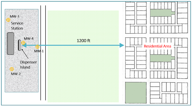
In this scenario, there has been a gasoline release from the dispenser island at a service station. While the leak is repaired shortly after the release, regulators and residents are worried about the release of benzene to the ground considering a residential development is located 1,200 feet to the east where shallow domestic wells are located. An initial on-site investigation reveals the following information:

• Aquifer material = medium sand; some gravel; little silt

• Hydraulic gradient to the east = 0.003 ft/ft

• Source area (MW-4) benzene concentration = 3,000 ug/L

Figure 1. Site map showing the distance from the benzene source at the dispenser island to the residential area.

Concerned by cleanup costs, the responsible party would prefer to remediate the contaminated area using MNA if possible. For MNA to be applicable, the responsible party needs to demonstrate that benzene is being flushed away sufficiently so as not to impact the domestic wells 1,200 feet away. For this example project, the benzene plume boundary is set to 5 ug/L since the USEPA drinking water standard for benzene is 5 ug/L.

Setting Up the Model

Since the leak from the dispenser island has been repaired, there is no constant source of contamination. Because of this, BIOSCREEN-AT is a good model solution for this analysis because its vertical patch source (in a semi-infinite aquifer bounded at the water table)  represents an exponentially decaying source concentration. This model solution will allow you to see changes in maximum plume extent from an early phase of growth, and then through subsequent plume decrease as the sources flushes away. In TS-CHEM, the following model parameters should be set:

• Hydraulic gradient = 0.003 ft/t

• Hydraulic conductivity = 60 ft/d

• Effective porosity = 0.25

• Source width = 10 ft

• Source depth = 2 ft

• Initial Benzene source concentration = 3,000 ug/L

• Initial estimate of source flushing half life = 4 years

Analysis 1: Examining Source Decrease Through Flushing

First, model observation points should be set downgradient from the dispenser at 100 ft (MW-1), 600 ft (mid-way to the neighborhood), and 1000 ft (approaching the neighborhood).

Figure 2. Site map showing model observation points located in between the dispenser island and the residential area.

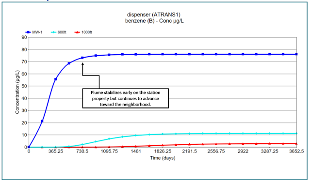
These observation points should give insight into the levels of benzene at these locations over time and whether the benzene plume is decaying at a sufficient rate. After running the model for ten years, the C v t plots reveal that the plume reaches a peak around 1.5 years on the station property but continues to advance towards the neighborhood. The observation points located farther downgradient from the source show the arrival and growth (increasing concentrations) of the plume until the reduction of the source causes concentrations to decline in these areas.

Figure 3. The C v t chart in TS-CHEM displaying benzene concentrations near the source at MW-1 (dark blue), 600 ft from the source (aqua), and 1000 ft from the source (red).

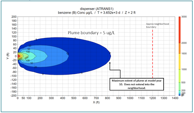
The contour plot shows that the plume reaches its maximum extent of about 875 feet after 7 years and does not extend into the residential development. The calculated plume at the 7-year time point encompasses an area of  88,350 ft².

Figure 4. TS-CHEM's contour chart indicates that the maximum plume extent (bound at 5 ug/L) does not reach the residential area.

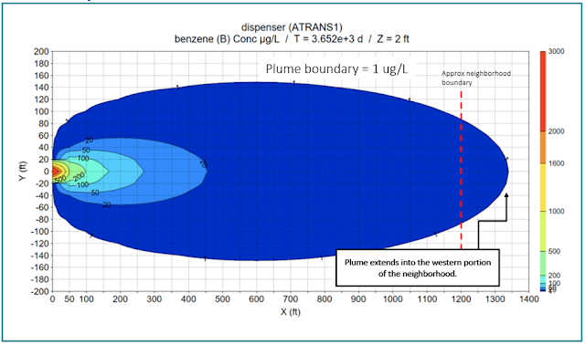
The contour plot set to year 10 shows that the extent of the benzene plume shrinks by about 150 feet. The plume will continue to shrink slowly over many years until it decreases below the 5 ug/L standard. Due to this slow rate of decay, a decision may be made to either move to evaluating an active remedy scenario in which the source is removed, or possibly to evaluate a scenario with a more rapid rate of source depletion. That source depletion Analysis 2 is presented below.

Figure 5. TS-CHEM's contour chart showing a reduction in plume extent from year 7 to year 10.

Analysis 2: Examining a Higher Source Degradation Rate

Let’s say that the responsible party continues to investigate the source area of the contamination and develops information that supports a Conceptual Site Model in which the source is depleting more rapidly. Instead of the 4-year half-life employed in the previous analysis, let’s change the source decay rate to a two year half-life, and observe the effects. After running the model with this new degradation rate, the C v t plot shows a faster depletion of benzene overall as well as a faster concentration decline.

Figure 6. The C v t chart in TS-CHEM displaying benzene concentrations at the three set observation points.

The contour chart shows that after 6 years, the benzene plume (with a boundary of 5 ug/L) extends about 810 feet with an area of 68,150 ft2 before receding, which is 22% smaller than the maximum plume extent in the previous analysis. By year 10, the plume boundary recedes to about 220 feet.

Figure 7. The contour chart in TS-CHEM set to year 6 highlighting its shorter plume extent compared to the previous analysis.

The smaller plume area and quick recession of the plume may support the case for MNA at this site. Further source zone characterization may be needed to support the use of the faster degradation rate, however.

Analysis 3: Examining A Higher Source and Plume Degradation Rate

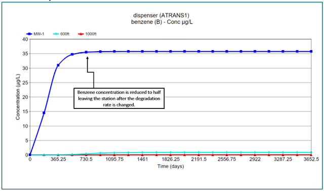
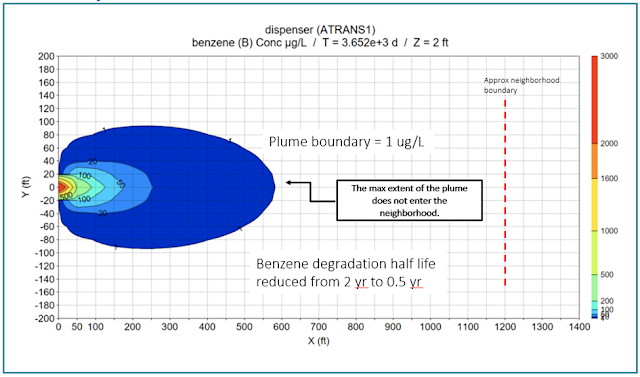
Oftentimes, regulatory agencies prescribe longer half-lives for constituents for the purposes of risk evaluations. In many cases, however, half-lives of contaminants like benzene are shorter than the default degradation rates typically prescribed by regulatory agencies. In this analysis, let’s increase the degradation rate of the plume (in addition to the increased degradation rate of the source in the last analysis) to observe the contamination extent in the case of a rapidly depleting source and plume. Instead of a 2-year half-life, let’s change the benzene degradation rate to a 0.5 year half-life.

The C v t plot shows that the maximum concentration observed at MW-1 is less than the maximum concentrations observed in the previous two analyses. Also, the plume decays before reaching the next two observation points at 600 and 1000 feet.

Figure 8. The TS-CHEM C v t chart showing benzene concentrations in the three set observation points. In this analysis, benzene isn't detected at the latter two observation points.

The benzene plume extends to about 350 feet after 2 years before quickly shrinking in areal extent. The plume area at year 2 is 26,150 ft², which is 61% smaller than the maximum plume extent in the first analysis. After year 10, the plume only extends to about 110 feet due to the groundwater flushing of the source, as well as the higher degradation occurring within the plume itself.

Figure 9. A greatly reduced benzene plume seen in TS-CHEM's contour chart following the increase of plume and source degradation rates.

This analysis - - especially using the more rapid benzene plume degradation rate - - shows that MNA could be a good potential remedial option for this site if acceptable information can be generated to support the degradation rates of the source and the plume. 

Conclusion

MNA is an attractive remedial option for parties looking to reduce cleanup costs, however, it must first be demonstrated that your site is a viable candidate for MNA per state and federal guidance. This often includes using data-driven solutions to form lines of evidence as to why your site is suitable for MNA. TS-CHEM provides a simple tool to evaluate the growth and decay of a contaminant plume, which allows for the evaluation of potential impacts to receptor locations downgradient from the source in the case the source concentration decreases through time due to flushing. This type of analysis can help determine a site’s suitability for MNA as a remedy.

TS-CHEM Example Applications – Receptor Impact Assessment

TS-CHEM is not only simple and easy to use, but it can be applied to a number of different common  situations when it comes to impacted  groundwater, making it the perfect tool for environmental professionals who perform groundwater investigation and remediation activities. To show how TS-CHEM can be used to evaluate a number of common groundwater issues, we have created a series of Example Applications.  In this blog post, we introduce the first Example Application in the series, which demonstrates how TS-CHEM can be used to model the length of a contaminant plume (in this case a benzene plume) in order to determine if it will impact domestic wells at a nearby residential development. You can download the model files and accompanying overview slide deck for the example application described below HERE.

 

Overview

In Example Application 1, there has been a small leak beneath a dispenser island at a gasoline station. This leak has led to a release of benzene into the groundwater below the site with the source concentrated near monitoring well MW-4. A residential development is located 1200 ft (1/4 mile) away from the leak location, and there is concern as to whether domestic wells may be impacted by benzene.  TS-CHEM can be utilized to determine whether the dissolved benzene plume from the dispenser release will reach the domestic wells above the drinking water standard of 5 ug/L.

Fig 1. Site map showing the distance from the benzene source at the dispenser island to the residential area. 

Setting up The Model

Considering the benzene release recently occurred and no remediation has taken place yet, we want to treat the contamination source as constant source rather than a decaying or transient source. Therefore, ATRANS1 is the perfect model solution for this scenario since it is a continuous and constant source model, and it will allow for a conservative evaluation of the maximum extent of the benzene plume.

Once we’ve chosen ATRANS1 as our model solution, we need to input all of the necessary model parameters that have been measured or estimated from a preliminary investigation of the station, as shown below:

• Hydraulic gradient = 0.003 ft/ft
• Hydraulic conductivity = 60 ft/d
• Effective porosity = 0.25
• Benzene source concentration = 3,000 ug/L
• Source width (width of dispenser island) = 10 ft
• Source depth (smear zone thickness beneath water table) = 2 ft

 

Analysis 1

First, we set two model observation points downgradient from the source at 600 ft and 1000 ft away. This will allow us to view the rise and stabilization of the benzene plume at these locations. Next, we run the model for a duration of 10 years. Once the model is finished running, we can display the concentration versus time (C v t) chart:

Fig 2. The C v t chart in TS-CHEM displaying benzene concentrations near the source at MW-1 (dark blue), 600 ft from the source (aqua), and 1000 ft from the source (red).

The dark blue line shows that benzene concentrations at MW-1 where groundwater leaves the station property stabilize at around 76 ug/L, while our observation points we set at 600 ft and 1000 ft show benzene concentrations stabilizing around 11 ug/L and 3 ug/L, respectively. This chart shows how the stabilized concentration of benzene decreases as you move further away from the gas station.

Now, let’s take a look at our contour chart set to model year 10:

Fig 3. TS-CHEM’s contour chart indicates that the maximum plume extent (bound at 5 ug/L) does not reach the residential area.

In the chart above, we’ve set the plume boundary to 5 ug/L, which in this example, is the applicable drinking water standard for benzene. Notice how the maximum extent of the plume does not reach the neighborhood under these model conditions. In this case, one might conclude that based on the results of the analysis, the benzene contamination at the gas station does not impact receptors (domestic wells).

Analysis 2

As noted above, the initial analyses performed using ATRANS 1 indicate that groundwater concentrations are not likely to reach downgradient receptor wells above 5 ug/L. However, let’s say that local regulations impose a different standard, and we must now evaluate a drinking water standard for benzene of 1 ug/L. Accordingly, we will need to perform an additional analysis to evaluate whether downgradient receptor wells may be impacted at concentrations above 1 ug/L.

Since nothing at our site has changed (including aquifer characteristics, source concentrations, and source size), we just have to adjust our outer plume contour from 5 ug/L to 1 ug/L. Once we’ve changed the plume contour, we can re-examine the contour chart at model year ten:

Fig 4. TS-CHEM’s contour chart indicates that the benzene plume, with a boundary of 1 ug/L, will impact the residential area.

As shown in Figure 4 above, the plume visibly extends much further to the east than it did in Analysis 1 (Figure 3), and therefore, our conclusion has changed; under this more stringent drinking water standard, the benzene spill at the gas station may impact downgradient receptors. But as noted above, these analyses are very conservative.  What if more reasonable inputs are used?

Analysis 3

Oftentimes, regulatory agencies prescribe longer half lives for constituents for the purposes of risk evaluations. In many cases, however, half-lives of contaminants like benzene are shorter than the default degradation rates typically prescribed by regulatory agencies. In our last two analyses, we used the default degradation rate of 9.58E-04 d^-1 (half life = 2 years). Let’s change the degradation rate to a more realistic value of 3.8E-03 d^-1 (half life = 0.5 years). After running the model again, there is a noticeable difference in the concentration and length of the benzene plume.

Fig 5. The C v t chart in TS-CHEM shows that benzene concentrations stabilize at a much lower level when the degradation rate is increased.

As shown in Figure 5 above, the C v t chart shows that benzene stabilizes around 35 ug/L at MW-1 near the station property boundary, which is about half the concentration observed in the previous analyses. Additionally, the benzene barely registers at our downgradient observation points. Now let’s look at the contour chart to examine the maximum extent of the plume using this higher degradation rate.

Fig 6. The contour chart demonstrates the effect of increasing the degradation rate of benzene. The plume, while still bound at the more protective 1 ug/L, no longer impacts the residential area.

Review of contour charts for each model year indicates that the benzene plume stabilizes in less than 4 years, which is about half the time it took the plume to stabilize in the previous analyses. Also, the plume, bound at 1 ug/L, reaches a maximum length of approximately 580 ft, and thus, does not impact the neighborhood domestic wells. The length of the benzene plume observed in this analysis is consistent with benzene plume lengths seen in many literature studies such as API 1998 and Connor et al 2014.

Why is this important?

In the case of a leak or spill of hazardous substances, government agencies may require some form of receptor impact evaluation in order to protect people and ecological receptors from exposure to contamination. TS-CHEM is a quick and easy, and science-base, way for any environmental professional to assess potential risks to receptors, evaluate the effect of changes in input parameters, and support decisions regarding the possible need for remedial actions. With over 30 solution models to choose from and a library of the most commonly modeled constituents, you can select an appropriate model and quickly (and easily) perform a receptor impact evaluation at your site!

To learn more about TS-CHEM, or to download a FREE DEMO of the software, visit the TS-CHEM Website! If you would like to see what else TS-CHEM can do, check out our other Example Applications!