TS-CHEM Example Applications – Receptor Impact Assessment

TS-CHEM is not only simple and easy to use, but it can be applied to a number of different common  situations when it comes to impacted  groundwater, making it the perfect tool for environmental professionals who perform groundwater investigation and remediation activities. To show how TS-CHEM can be used to evaluate a number of common groundwater issues, we have created a series of Example Applications.  In this blog post, we introduce the first Example Application in the series, which demonstrates how TS-CHEM can be used to model the length of a contaminant plume (in this case a benzene plume) in order to determine if it will impact domestic wells at a nearby residential development. You can download the model files and accompanying overview slide deck for the example application described below HERE.

 

Overview

In Example Application 1, there has been a small leak beneath a dispenser island at a gasoline station. This leak has led to a release of benzene into the groundwater below the site with the source concentrated near monitoring well MW-4. A residential development is located 1200 ft (1/4 mile) away from the leak location, and there is concern as to whether domestic wells may be impacted by benzene.  TS-CHEM can be utilized to determine whether the dissolved benzene plume from the dispenser release will reach the domestic wells above the drinking water standard of 5 ug/L.

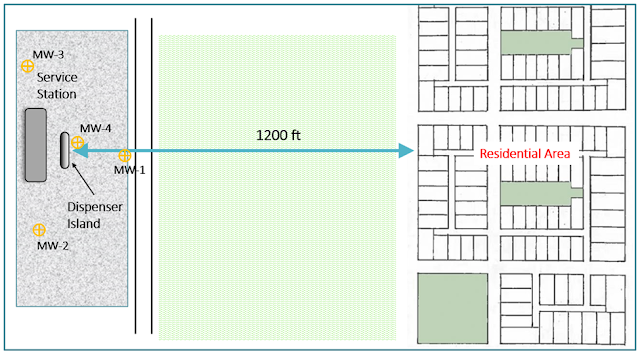Fig 1. Site map showing the distance from the benzene source at the dispenser island to the residential area. 

Setting up The Model

Considering the benzene release recently occurred and no remediation has taken place yet, we want to treat the contamination source as constant source rather than a decaying or transient source. Therefore, ATRANS1 is the perfect model solution for this scenario since it is a continuous and constant source model, and it will allow for a conservative evaluation of the maximum extent of the benzene plume.

Once we’ve chosen ATRANS1 as our model solution, we need to input all of the necessary model parameters that have been measured or estimated from a preliminary investigation of the station, as shown below:

• Hydraulic gradient = 0.003 ft/ft
• Hydraulic conductivity = 60 ft/d
• Effective porosity = 0.25
• Benzene source concentration = 3,000 ug/L
• Source width (width of dispenser island) = 10 ft
• Source depth (smear zone thickness beneath water table) = 2 ft

 

Analysis 1

First, we set two model observation points downgradient from the source at 600 ft and 1000 ft away. This will allow us to view the rise and stabilization of the benzene plume at these locations. Next, we run the model for a duration of 10 years. Once the model is finished running, we can display the concentration versus time (C v t) chart:

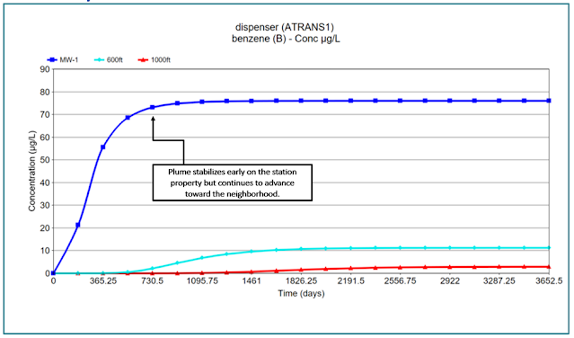Fig 2. The C v t chart in TS-CHEM displaying benzene concentrations near the source at MW-1 (dark blue), 600 ft from the source (aqua), and 1000 ft from the source (red).

The dark blue line shows that benzene concentrations at MW-1 where groundwater leaves the station property stabilize at around 76 ug/L, while our observation points we set at 600 ft and 1000 ft show benzene concentrations stabilizing around 11 ug/L and 3 ug/L, respectively. This chart shows how the stabilized concentration of benzene decreases as you move further away from the gas station.

Now, let’s take a look at our contour chart set to model year 10: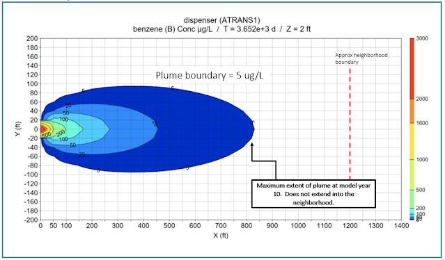

Fig 3. TS-CHEM’s contour chart indicates that the maximum plume extent (bound at 5 ug/L) does not reach the residential area.

In the chart above, we’ve set the plume boundary to 5 ug/L, which in this example, is the applicable drinking water standard for benzene. Notice how the maximum extent of the plume does not reach the neighborhood under these model conditions. In this case, one might conclude that based on the results of the analysis, the benzene contamination at the gas station does not impact receptors (domestic wells).

Analysis 2

As noted above, the initial analyses performed using ATRANS 1 indicate that groundwater concentrations are not likely to reach downgradient receptor wells above 5 ug/L. However, let’s say that local regulations impose a different standard, and we must now evaluate a drinking water standard for benzene of 1 ug/L. Accordingly, we will need to perform an additional analysis to evaluate whether downgradient receptor wells may be impacted at concentrations above 1 ug/L.

Since nothing at our site has changed (including aquifer characteristics, source concentrations, and source size), we just have to adjust our outer plume contour from 5 ug/L to 1 ug/L. Once we’ve changed the plume contour, we can re-examine the contour chart at model year ten: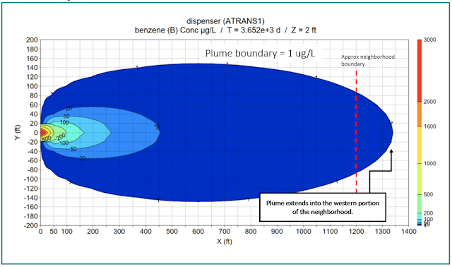

Fig 4. TS-CHEM’s contour chart indicates that the benzene plume, with a boundary of 1 ug/L, will impact the residential area.

As shown in Figure 4 above, the plume visibly extends much further to the east than it did in Analysis 1 (Figure 3), and therefore, our conclusion has changed; under this more stringent drinking water standard, the benzene spill at the gas station may impact downgradient receptors. But as noted above, these analyses are very conservative.  What if more reasonable inputs are used?

Analysis 3

Oftentimes, regulatory agencies prescribe longer half lives for constituents for the purposes of risk evaluations. In many cases, however, half-lives of contaminants like benzene are shorter than the default degradation rates typically prescribed by regulatory agencies. In our last two analyses, we used the default degradation rate of 9.58E-04 d^-1 (half life = 2 years). Let’s change the degradation rate to a more realistic value of 3.8E-03 d^-1 (half life = 0.5 years). After running the model again, there is a noticeable difference in the concentration and length of the benzene plume.

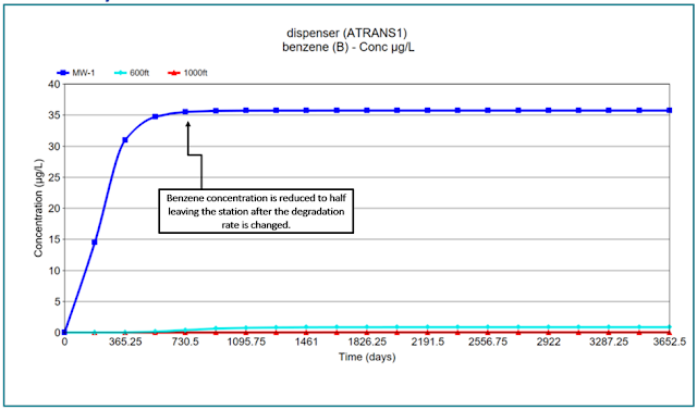Fig 5. The C v t chart in TS-CHEM shows that benzene concentrations stabilize at a much lower level when the degradation rate is increased.

As shown in Figure 5 above, the C v t chart shows that benzene stabilizes around 35 ug/L at MW-1 near the station property boundary, which is about half the concentration observed in the previous analyses. Additionally, the benzene barely registers at our downgradient observation points. Now let’s look at the contour chart to examine the maximum extent of the plume using this higher degradation rate.

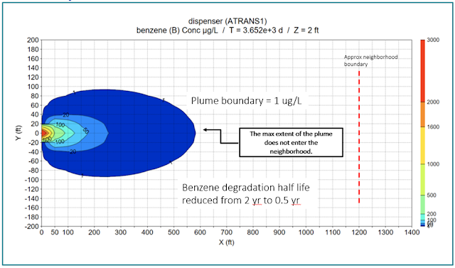Fig 6. The contour chart demonstrates the effect of increasing the degradation rate of benzene. The plume, while still bound at the more protective 1 ug/L, no longer impacts the residential area.

Review of contour charts for each model year indicates that the benzene plume stabilizes in less than 4 years, which is about half the time it took the plume to stabilize in the previous analyses. Also, the plume, bound at 1 ug/L, reaches a maximum length of approximately 580 ft, and thus, does not impact the neighborhood domestic wells. The length of the benzene plume observed in this analysis is consistent with benzene plume lengths seen in many literature studies such as API 1998 and Connor et al 2014.

Why is this important?

In the case of a leak or spill of hazardous substances, government agencies may require some form of receptor impact evaluation in order to protect people and ecological receptors from exposure to contamination. TS-CHEM is a quick and easy, and science-base, way for any environmental professional to assess potential risks to receptors, evaluate the effect of changes in input parameters, and support decisions regarding the possible need for remedial actions. With over 30 solution models to choose from and a library of the most commonly modeled constituents, you can select an appropriate model and quickly (and easily) perform a receptor impact evaluation at your site!

To learn more about TS-CHEM, or to download a FREE DEMO of the software, visit the TS-CHEM Website! If you would like to see what else TS-CHEM can do, check out our other Example Applications!