TS-CHEM Example Applications – Receptor Impact Assessment

TS-CHEM is not only simple and easy to use, but it can be applied to a number of different common  situations when it comes to impacted  groundwater, making it the perfect tool for environmental professionals who perform groundwater investigation and remediation activities. To show how TS-CHEM can be used to evaluate a number of common groundwater issues, we have created a series of Example Applications.  In this blog post, we introduce the first Example Application in the series, which demonstrates how TS-CHEM can be used to model the length of a contaminant plume (in this case a benzene plume) in order to determine if it will impact domestic wells at a nearby residential development. You can download the model files and accompanying overview slide deck for the example application described below HERE.

 

Overview

In Example Application 1, there has been a small leak beneath a dispenser island at a gasoline station. This leak has led to a release of benzene into the groundwater below the site with the source concentrated near monitoring well MW-4. A residential development is located 1200 ft (1/4 mile) away from the leak location, and there is concern as to whether domestic wells may be impacted by benzene.  TS-CHEM can be utilized to determine whether the dissolved benzene plume from the dispenser release will reach the domestic wells above the drinking water standard of 5 ug/L.

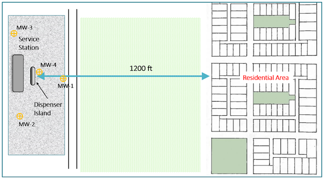
Fig 1. Site map showing the distance from the benzene source at the dispenser island to the residential area. 

Setting up The Model

Considering the benzene release recently occurred and no remediation has taken place yet, we want to treat the contamination source as constant source rather than a decaying or transient source. Therefore, ATRANS1 is the perfect model solution for this scenario since it is a continuous and constant source model, and it will allow for a conservative evaluation of the maximum extent of the benzene plume.

Once we’ve chosen ATRANS1 as our model solution, we need to input all of the necessary model parameters that have been measured or estimated from a preliminary investigation of the station, as shown below:

• Hydraulic gradient = 0.003 ft/ft
• Hydraulic conductivity = 60 ft/d
• Effective porosity = 0.25
• Benzene source concentration = 3,000 ug/L
• Source width (width of dispenser island) = 10 ft
• Source depth (smear zone thickness beneath water table) = 2 ft

 

Analysis 1

First, we set two model observation points downgradient from the source at 600 ft and 1000 ft away. This will allow us to view the rise and stabilization of the benzene plume at these locations. Next, we run the model for a duration of 10 years. Once the model is finished running, we can display the concentration versus time (C v t) chart:

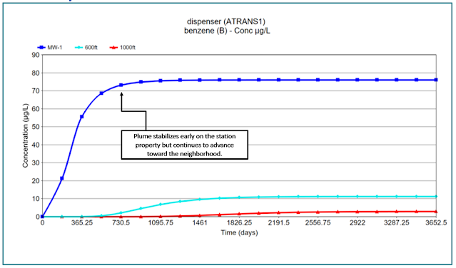
Fig 2. The C v t chart in TS-CHEM displaying benzene concentrations near the source at MW-1 (dark blue), 600 ft from the source (aqua), and 1000 ft from the source (red).

The dark blue line shows that benzene concentrations at MW-1 where groundwater leaves the station property stabilize at around 76 ug/L, while our observation points we set at 600 ft and 1000 ft show benzene concentrations stabilizing around 11 ug/L and 3 ug/L, respectively. This chart shows how the stabilized concentration of benzene decreases as you move further away from the gas station.

Now, let’s take a look at our contour chart set to model year 10:

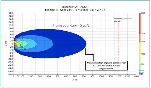
Fig 3. TS-CHEM’s contour chart indicates that the maximum plume extent (bound at 5 ug/L) does not reach the residential area.

In the chart above, we’ve set the plume boundary to 5 ug/L, which in this example, is the applicable drinking water standard for benzene. Notice how the maximum extent of the plume does not reach the neighborhood under these model conditions. In this case, one might conclude that based on the results of the analysis, the benzene contamination at the gas station does not impact receptors (domestic wells).

Analysis 2

As noted above, the initial analyses performed using ATRANS 1 indicate that groundwater concentrations are not likely to reach downgradient receptor wells above 5 ug/L. However, let’s say that local regulations impose a different standard, and we must now evaluate a drinking water standard for benzene of 1 ug/L. Accordingly, we will need to perform an additional analysis to evaluate whether downgradient receptor wells may be impacted at concentrations above 1 ug/L.

Since nothing at our site has changed (including aquifer characteristics, source concentrations, and source size), we just have to adjust our outer plume contour from 5 ug/L to 1 ug/L. Once we’ve changed the plume contour, we can re-examine the contour chart at model year ten:

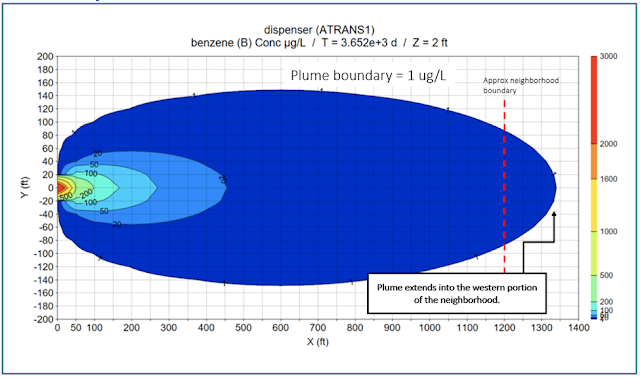
Fig 4. TS-CHEM’s contour chart indicates that the benzene plume, with a boundary of 1 ug/L, will impact the residential area.

As shown in Figure 4 above, the plume visibly extends much further to the east than it did in Analysis 1 (Figure 3), and therefore, our conclusion has changed; under this more stringent drinking water standard, the benzene spill at the gas station may impact downgradient receptors. But as noted above, these analyses are very conservative.  What if more reasonable inputs are used?

Analysis 3

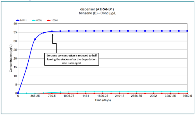
Oftentimes, regulatory agencies prescribe longer half lives for constituents for the purposes of risk evaluations. In many cases, however, half-lives of contaminants like benzene are shorter than the default degradation rates typically prescribed by regulatory agencies. In our last two analyses, we used the default degradation rate of 9.58E-04 d^-1 (half life = 2 years). Let’s change the degradation rate to a more realistic value of 3.8E-03 d^-1 (half life = 0.5 years). After running the model again, there is a noticeable difference in the concentration and length of the benzene plume.

Fig 5. The C v t chart in TS-CHEM shows that benzene concentrations stabilize at a much lower level when the degradation rate is increased.

As shown in Figure 5 above, the C v t chart shows that benzene stabilizes around 35 ug/L at MW-1 near the station property boundary, which is about half the concentration observed in the previous analyses. Additionally, the benzene barely registers at our downgradient observation points. Now let’s look at the contour chart to examine the maximum extent of the plume using this higher degradation rate.

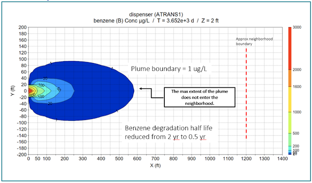
Fig 6. The contour chart demonstrates the effect of increasing the degradation rate of benzene. The plume, while still bound at the more protective 1 ug/L, no longer impacts the residential area.

Review of contour charts for each model year indicates that the benzene plume stabilizes in less than 4 years, which is about half the time it took the plume to stabilize in the previous analyses. Also, the plume, bound at 1 ug/L, reaches a maximum length of approximately 580 ft, and thus, does not impact the neighborhood domestic wells. The length of the benzene plume observed in this analysis is consistent with benzene plume lengths seen in many literature studies such as API 1998 and Connor et al 2014.

Why is this important?

In the case of a leak or spill of hazardous substances, government agencies may require some form of receptor impact evaluation in order to protect people and ecological receptors from exposure to contamination. TS-CHEM is a quick and easy, and science-base, way for any environmental professional to assess potential risks to receptors, evaluate the effect of changes in input parameters, and support decisions regarding the possible need for remedial actions. With over 30 solution models to choose from and a library of the most commonly modeled constituents, you can select an appropriate model and quickly (and easily) perform a receptor impact evaluation at your site!

To learn more about TS-CHEM, or to download a FREE DEMO of the software, visit the TS-CHEM Website! If you would like to see what else TS-CHEM can do, check out our other Example Applications!

1-D vs 3-D Transport Analysis of Contaminant Plume Extent

 A 1-D analysis of contaminant transport often greatly overestimates plume extent, resulting in an overly-conservative assessment.

A common question related to contaminant plumes: “How far downgradient will the plume extend?”

We may want to know this for several reasons:

•       Will the plume reach a receptor at some distance from the source?

•       How far should I place monitoring wells to measure the plume?

•       And in some states (e.g. NJ) how far should I draw the boundary of the groundwater Classification Exception Area (CEA).

Possible Methods

To analyze plume extent from the source over time, we can perform screening analyses using models ranging from simple analytic 1-D solutions, to 3-D analytic and semi-analytic solutions. We could also use more costly and sophisticated 3-D numerical fate and transport models - - but to examine the difference between a 1-D model and a 3-D model, analytical solutions are perfectly capable analysis tools.

1-D Plume Transport Modeling

For many decades, from the 1970s through present, investigators and regulators have often explored the movement of a dissolved chemical plume extending downgradient from a steadily-releasing source using some form of mathematical solution to the 1-D transport equation (e.g. Ogata and Banks 1961; Bear 1972 & 1979). The often cited Ogata and Banks 1961 solution is a simple representation of advective-dispersive transport that does not incorporate the processes of adsorption (retardation) nor degradation. The Bear 1972 & 1979 solutions are more useful because they incorporate the effects of dispersion, retardation, and degradation.

1-D Example Application 

To illustrate the plume length that a 1-D model would calculate, a simple example was developed in which the Bear 1-D transport solution was used to calculate the location of the 5 ug/L plume boundary of a benzene plume 5880 days (16 years) after release (Fig 1). Source benzene concentration was assumed to remain constant at 1000 ug/L; groundwater velocity was set to 1 ft/d and retardation factor was set to 2; 1-D aquifer dispersivity was 50 ft; and a conservative benzene plume half-life of 2 years was applied. 

Fig 1. 1-D calculation shows plume extends 2900 ft from the source after 5880 days.

3-D Plume Transport Modeling

Another approach often employed by investigators or regulators is to begin with the full 3-D transport equation and apply that 3-D solution to calculate concentration along the centerline of the plume to determine the extent of the plume in the downgradient direction.

One of the widely known solutions to the 3-D transport equations was developed by Domenico in 1987. This solution forms the basis for a number of models used by regulatory agencies to estimate contaminant plume movement:

•     BIOSCREEN developed by USEPA (see USEPA website for BIOSCREEN v1.4)

•     BIOCHLOR (USEPA) v 2.2

•     Quick Domenico model described by PADEP in certain of its regulatory documents (see PADEP website Quick Domenico spreadsheet model)

3-D Example Application 

So, we can now solve the same plume transport problem illustrated in Fig 1, but we will instead use the 3-D Domenico solution model (instead of 1-D). Transverse dispersivity is set to 1/10^th the longitudinal dispersivity and vertical dispersivity is set to 1/1000^th the longitudinal dispersivity (these parameters were not present in the 1-D model). The 3-D transport solution calculates a much shorter plume length; 1280 ft versus the 1-D length of 2900 ft (Fig 2).

Fig 2. 3-D calculation shows plume extends 1280 ft from the source after 5880 days.

Newer 3-D Methods

Analytical

In recent years minor discrepancies have been reported between the Domenico solution and more rigorous solutions to the 3-D transport equations (see for example (Guyonnet and Neville 2004; West et al 2007; Srinivasan et al 2007; Karanovic et al 2007; Devlin et al 2012). The discrepancies occur primarily along the centerline axis of the plume; this means that errors may be introduced when attempting to estimate the plume length (i.e. how far downgradient from the source contamination may extend).

Several investigators have modified the original Domenico 3-D transport solution to attempt to mitigate the errors caused by the original formulation. For example:

•     BIOSCREEN (USEPA) was updated to BIOSCREEN-AT (Karanovic & Neville 2007)

•     Srinivasan, Clement & Lee (2007) published an updated version of the Domenico solution

Semi-Analytical

The 1-D and 3-D solutions we have examined to this point are analytic solutions. Certain simplifications are made in the formulation of the transport differential equation that allows it to be solved in closed form - - i.e. the solution does not contain an integral term; the algebraic equation can be solved in a spreadsheet

There is a class of more rigorous solutions that are not simplified and still contain an integral term; and because of that, they are more accurate. These solutions are typically solved in a simple program that employs a numerical integration routine to arrive at the calculated concentrations.

Examples of these semi-analytical transport models include:

•       ATRANS

•       BIOSCREEN-AT (Domenico 1987 solution modified by Karanovic et al 2007)

•       3DADE (USDA 1994)

•       N3DADE (USDA 1997)

•       AT123D-AT (Yeh 1984 solution modified by Burnell et al 2012)

These solutions have been assembled into a unified user interface in TS-CHEM. They provide a means of calculating more accurate estimates of contaminant plume extent for environmental assessments.

To summarize: Contaminant plume analyses based on 1-D models are likely to greatly overestimate plume extent. This may result in an overly-conservative assessment that causes concern, or results in actions, related to impacts that are not likely to occur. More accurate evaluations of plume extent can be calculated using 3-D contaminant transport model. TS-CHEM provides a library of over 30 analytical 3D plume transport solutions for making these types of evaluations.

To learn more about TS-CHEM, or to download a FREE DEMO VERSION of the software, visit the TS-CHEM Website today!

 

TS-CHEM Solution Library - ATRANS

The TS-CHEM program includes a comprehensive library of more than 30 different analytical solutions, each with different capabilities, including how they represent contaminant sources. For this first post in the Solution Library series, we will be focusing on the ATRANS family of models developed by Chris Neville at SS Papadopulos & Associates. In fact, the ATRANS1 model is included in the DEMO version of TS-CHEM, so you can try it out for yourself at any time!

 

What is ATRANS?

ATRANS is a suite of analytical model solutions that are used to simulate three-dimensional advective-dispersive transport from a patch source along the inflow boundary of an aquifer, as show in the conceptual model below:

Figure 1 - ATRANS conceptual model

TS-CHEM includes all four ATRANS models: ATRANS1, ATRANS2, ATRANS3 and ATRANS4. All ATRANS models are based on the following key assumptions:

• Finite aquifer bounds (semi-finite in the x-direction, finite in the z-direction)
•  This essentially places no-mass-flux boundaries on the upper water-table boundary and the lower aquifer base boundary
• Uniform one-dimensional flow along the x-axis
• First-order reaction kinetics (e.g. biodegradation)
• Chemical sorption onto the aquifer material
• Rectangular patch source areas with user-specified concentration

What is the difference between the ATRANS models in the ATRANS package?

The main difference between the different ATRANS models is in how they handle the source concentrations over time. Taking from the Model Features Table located in Appendix D of the TS-CHEM User Guide we can see that in the ATRANS models the source can either be constant, decaying, or transient (time varying):

Solution Model	Source vs Time
	Constant Source	Decaying Source	Transient Source
ATRANS1	X
ATRANS2		X
ATRANS3			X
ATRANS4			X

With this table in mind, we can take a visual look at how these sources are represented with figures of concentration over time from the ATRANS user manual and the Model Selection Tool in TS-CHEM:

Figure 2 - ATRANS model inputs: source concentrations over time

You may have noticed that ATRANS3 and ATRANS4 both handle transient (time-variable) source concentrations. The difference between these two models is in how the transient concentration data is introduced to the model. ATRANS3 asks the user to input a series of time-concentration pairs that define the source concentration history (for example from measured values at certain points in time.  The software then creates discrete time steps with histograms that mimic the continuous data, with the specified concentration point at the center of each histogram bar. ATRANS4 asks the user to input a series of time-concentration pairs, but for this model the user is specifying the concentration level at the start of a histogram bar that remains in effect until the next starting time and concentration is specified (for example from historical knowledge of the starts of spills or releases at a site source at certain points in time).

What applications are the ATRANS models best suited for?

As discussed in the previous blog post “TS-CHEM – The Swiss-Army Knife of Solute Transport Modeling” environmental professionals are often tasked with developing conceptual site models (CSMs) that characterize the extent and behavior of groundwater contaminant plumes, which the ATRANS models can assist with. In particular, the ATRANS models are useful for representing sites where the aquifer thickness is known or is believed to be bounded at a finite depth by an impermeable base (finite aquifer boundary)and where the investigator has information on concentration at the downgradient edge of a source area (patch source). If only a single source concentration is known, and/or the investigator wished to perform a conservative analysis, a constant source ATRANS1 model can be applied. If the source is understood to be flushing and depleting through time, an exponentially decaying ATRANS2 source model can be applied. And if information is available on the changing history (both increases and decreases) of source concentration with time, then an ATRANS3 or ATRANS4 model can be applied, as described further below.

 

The ATRANS1 model is useful for simulating scenarios that can be represented by constant concentration sources. For instance, it can be used to support remedial design by evaluating a conservative maximum plume extent and when the plume becomes stable. It can also be used for regulatory compliance by conservatively simulating potential receptor well impacts, or to assist with the delineation of groundwater Classification Exception Areas (CEAs).

Figure 3 - ATRANS1 solution showing maximum plume extent and stability for a benzene plume with a constant source at 200ft, 600ft and 1000ft from the source

The ATRANS2 model is useful for simulating scenarios that can be represented by an exponential decay in the source concentration and is one of three models in the TS-CHEM library that can do so (the others being BIOSCREEN-AT and BIOSCREEN-AT NI). For example, if an environmental professional wanted to simulate a scenario where a benzene plume from a small spill source that is flushing and degrading with time, they could use TS-CHEM and ATRANS2 with a decaying source to see how a Monitored Natural Attenuation (MNA) remedy would reduce plume concentrations over a ten-year period, particularly at locations close to the source:

Figure 4 - ATRANS2 solution showing benzene plume concentrations after natural source flushing and MNA at 200ft, 600ft and 1000ft from the source

The ATRANS3 and ATRANS4 models are two of only four solutions in the TS-CHEM library that can account for transient source concentrations (the others being AT123D-AT FT and AT123D-AT IT which differ from the ATRANS models in that AT123D-AT models employ mass flux specified sources in unbounded aquifers). The ability to have transient source concentrations allows for the simulation of intermittent single sources, multiple sources that occur at different (or overlapping) times, and even termination of a source as would result from a source removal remedy. In the example below, ATRANS4 was used to simulate effects on a benzene plume as a result of remedial activities, where the source was ceased after 180 days (to account for source removal as part of active remediation) and MNA was able to reduce the concentration of the plume to below 5 ug/L in the entire plume after just 2.5 years.

Figure 5 - ATRANS4 solution showing benzene plume concentrations after source remediation and MNA at 200ft, 600ft and 1000ft from the source

To summarize: the ATRANS family of models, which are built-in as part of the TS-CHEM solution library, allow for flexible representation of the source through time. The models assume a finite aquifer boundary, so they are ideal for bounded aquifer models. The choice of model will depend primarily on how the concentration of the simulated source changes over time, as ATRANS models allow for sources that are constant, exponentially decaying, or even time-variable. The ATRANS models allow environmental professionals to evaluate plume characteristics for a variety of groundwater plume transport scenarios.

To learn more about TS-CHEM, or to download a FREE DEMO VERSION of the software, visit the TS-CHEM Website today!

New Features in TS-CHEM Version 2022-3

 TS-CHEM v2022-3 has some great new features, including new options for BIOSCREEN-AT, Dark Mode (Mac version) and the ability to double-click project files to open them. But some of the most powerful features center around the new chart controls. A brief overview of these new chart controls is included below.

CHART AXIS CONTROLS

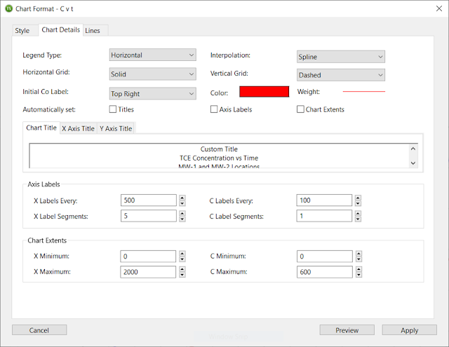
All three of the major chart types (C v t, Profile, and Contour) display axes; and so does the digitized concentration chart in the Concentration Inspector tool. In TS-CHEM v2022-3, the user can now control almost every aspect of the of these chart axes including:

• Major tick and label placement
• Minor tick spacing
• Chart grid lines
• Custom axis title
• Axis extent

Figure 1 - TS-CHEM Chart Axis Controls

These controls allow for the creation of better-looking data plots.

Figure 2 - TS-CHEM Concentration vs. Time Data Plot

And, in the case of the axis extent controls, they allow the user to zoom in on a portion of the chart to better examine data concentrations or trends.

Figure 3 - Zoom-in of TS-CHEM Data Plot

CONTOUR CHART CONTOLS

Contour charts now have a second set of controls (in addition to the axis controls) that allow easy formatting of the contour intervals and the type of contour chart used to display the data.

Intervals controls allow the user to accept the automatic TS-CHEM contouring, or specify Regular Intervals (min, max, and interval), or select Custom Contours to customize the spacing and color of the contour display. 

Figure 4 - TS-CHEM Contour Charts - Custom Settings

The value specified in the Boundary field (50 in the example above) serves as a plume cutoff concentration, and the plume image is transparent for concentrations below the Boundary value (see below). This makes it very easy to create a bounded plume to place on digital map using the Map Overlay feature.

Figure 5 - TCE Plume Contour Chart - Plume Bounded at 50 ppb

Additionally, the Style for a contour chart can be selected from a dropdown menu containing the following options:

• Fill – Color
• Fill – Grayscale
• Lines Only – Color
• Lines Only – Grayscale
• Lines Only – Black
  

An example of a Lines Only – Color contour chart is shown below.

Figure 6 - TCE Plume Contour Chart Displaying Lines Only - Plume Bounded at 50 ppb 

These sets of controls, tailored to each of the different chart types, provide the tools needed to produce report- or presentation-ready graphics from your TS-CHEM plume transport modeling analyses.

To learn more about the new features TS-CHEM v2022-3, or to download a FREE DEMO VERSION of the software, visit the TS-CHEM Website today